Curtis T McMullen 的 C 程式^[1]

如何執行

julia.tar

描述^[2]

步驟

執行 tcsh
make
將 ps2gif 指令碼複製到每個子目錄
將 ./ 新增到每個執行指令碼
執行

名稱

"大象的眼睛" 停留在主心形的內部角 p/q = 主 Misiurewicz 點

圖片

julia.tar
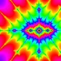在斐波那契點 c = -1.8705286321646448888906 處的曼德勃羅集
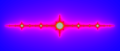飛機 Julia 集。C 是實軸上週期 3 分量的中心
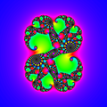
在週期 16 分量附近（尾流 1/16）的斷開連線的 Julia 集
來自尾流 1/19 的斷開連線的（康托爾）Julia 集

kleinian.tar
球體上的克萊因群極限集
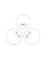平面上肖特基（克萊因）群極限集

程式碼

複數

// from cx.c  programs by Curtis T McMullen
// http://www.math.harvard.edu/~ctm/programs/home/prog/julia/src/julia.tar

/* Compute sqrt(z) in the half-plane perpendicular to w. */
complex contsqrt(z,w)
complex z,w;
{
	complex cx_sqrt(), t;

	t = cx_sqrt(z);
	if (0 > (t.x*w.x + t.y*w.y)) 
		{t.x = -t.x; t.y = -t.y;}
	return(t);
}


/* Values in [-pi,pi]. */
double arg(z)  
	complex z;
{
	return(atan2(z.y,z.x));
}


complex cx_exp(z)
	complex z;
{
	complex w;
	double m;

	m = exp(z.x);
	w.x = m * cos(z.y);
	w.y = m * sin(z.y);
	return(w);
}

complex cx_log(z)
	complex z;
{
	complex w;

	w.x = log(cx_abs(z));
	w.y = arg(z);
	return(w);
}

complex cx_sin(z)
	complex z;
{
	complex w;

	w.x = sin(z.x) * cosh(z.y);
	w.y = cos(z.x) * sinh(z.y);
	return(w);
}

complex cx_cos(z)
	complex z;
{
	complex w;

	w.x = cos(z.x) * cosh(z.y);
	w.y = -sin(z.x) * sinh(z.y);
	return(w);
}

complex cx_sinh(z)
	complex z;
{
	complex w;

	w.x = sinh(z.x) * cos(z.y);
	w.y = cosh(z.x) * sin(z.y);
	return(w);
}

complex cx_cosh(z)
	complex z;
{
	complex w;

	w.x = cosh(z.x) * cos(z.y);
	w.y = sinh(z.x) * sin(z.y);
	return(w);
}

complex power(z,t)   /* Raise z to a real power t */
	complex z;
	double t;
{	double arg(), cx_abs(), pow();
	complex polar();

	return(polar(pow(cx_abs(z),t), t*arg(z)));
}

/*  Map points in the unit disk onto the lower hemisphere of the
    Riemann sphere by inverse stereographic projection.
    Projecting, r -> s = 2r/(r^2 + 1);  inverting this,
    s -> r = (1 - sqrt(1-s^2))/s.   */
 
complex disk_to_sphere(z)
	complex z;
{       complex w;
        double cx_abs(), r, s, sqrt();
 
        s = cx_abs(z);
        if (s == 0) return(z);
                else r = (1 - sqrt(1-s*s))/s;
        w.x = (r/s)*z.x;
        w.y = (r/s)*z.y;
        return(w);
}

complex mobius(a,b,c,d,z)
        complex a,b,c,d,z;

{       return(divide(add(mult(a,z),b),
                   add(mult(c,z),d)));
}

逃逸時間和勢

// from quad.c  programs by Curtis T McMullen
// http://www.math.harvard.edu/~ctm/programs/home/prog/julia/src/julia.tar

/* F : \cx-K(f) -> {Re z > 0} is the multivalued
   function given by lim 2^{-n} log f^n(z).
   Re F(z) = rate, 
   (Re F(z))/|F'(z)| = dist.
   Returns 1 if z escaped, 0 otherwise.
*/

escape(z,c,iterlim,rate,dist)
	complex z,c;
	int iterlim;
	double *rate, *dist;
{
	int i;
	double fp, r, s;

	s = 1.0;
	fp = 1.0;
	for(i=0; i<iterlim; i++)
	{	r = cx_abs(z);
		if(r > LARGE)
		{	*rate = log(r)/s;
			*dist = r*log (r)/fp;
			return(1);
		}
		fp = fp * 2.0 * r;
		z = add(mult(z,z),c);
		s = s * 2.0;
	}
	return(0);
}

外部射線

// from quad.c  programs by Curtis T McMullen
// http://www.math.harvard.edu/~ctm/programs/home/prog/julia/src/julia.tar

/* CAUTION is 2^{1/n} */
#define LOG2 .69314718055994530941
#define SQRT2 1.414213562373095
#define LARGE 200.0
#define LENGTH 200
#define CAUTION 0.9330329915368074
#define CIRCLEPTS 1000
#define EPS 0.000001
#define RAYEPS 1e-20
#define JFAC 1.0

/* Defaults */
#define C {0, 1}
#define CENTER {0.0,0.0}
#define RADIUS 1.5
#define PCLIM 0
#define SUBDIVIDE 8
#define ITERLIM 50  


/* Analytically continue Riemann mapping */
/* F : unit disk -> \cx-K(f) */
/* Assuming F(r,ang) is approx. z, find exact value*/

complex riemann(r,ang,z)
	double r;
	rational ang;
	complex z;
{
	complex orb[LENGTH], neworb[LENGTH];
	int i, n;

	orb[0] = z;
	n = 0;
	for (i=0; i<LENGTH-1; i++)
	{	if(cx_abs(orb[i]) > LARGE) break;
		orb[i+1] =
		add(mult(orb[i],orb[i]),c);
		n++;
		r = 2*r;
		ang.num = (2*ang.num)%ang.den;
	}
	neworb[n] = polar(pow(2.0,r),2*PIVAL*ang.num/ang.den);

	for(i=n; i>0; i--)
	{	neworb[i-1] =
		contsqrt(sub(neworb[i],c),orb[i-1]);
	}
	return(neworb[0]);
}


/* Set the color on a line joining z to w */
scan_line(z,w,col)
	complex z, w;
	int col;
{	
	int i, n;
	complex u;

	n = 4*cx_abs(sub(z,w))/pixrad;
	if(n == 0)
	{	scan_set(z,col);
		return;
	}
	for(i=0; i<=n; i++)
	{	u.x = (i*z.x + (n-i)*w.x)/n; 	
		u.y = (i*z.y + (n-i)*w.y)/n; 	
		scan_set(u,col);
	}
}


/* Draw an external ray */
draw_ray(level,ang)
	double level;
	rational ang;
{
	complex lastz, z;
	double r;

	r = level;
	while(pow(2.0,r) < LARGE) r *= 2;
	z = polar(pow(2.0,r),2*PIVAL*ang.num/ang.den);
	do
	{	r = r*CAUTION;
		lastz = z;
		z = riemann(r,ang,lastz);
		if(r < level*0.99) 
			scan_line(lastz,z,RAY);
	} while(r > RAYEPS);
}

使用 Curtis McMullen 的逆 Boettcher 對映繪製動態外部射線

該方法基於 Curtis McMullen^[3] 的 C 程式及其由 Matjaz Erat^[4] 編寫的 Pascal 版本

這裡有兩個平面^[5]

w 平面（或 f0 平面）
z 平面（fc 平面的動態平面）

該方法包含 3 個主要步驟

計算圓的外部射線在 $f_{0}\,$ 平面上的某些 w 點，這些點對應於角度 $\theta \,$ 和不同的半徑（光柵化）

w_{0}=R*e^{2\pi it}\,

其中

1<R<\infty \,

使用逆 Boettcher 對映 $\Psi _{c}=\Phi _{c}^{-1}\,$ 將 w 點對映到 z 點

z_{0}=\Psi _{c}(w_{0})=f_{c}^{-n}(w_{0}^{2^{n}})\,

繪製 z 點（並使用線段連線它們（線段是直線上由兩個不同的端點界定的部分^[6]））

第一步和最後一步很簡單，但第二步並非如此，需要更多解釋。

光柵化

對於 $f_{0}\,$ 平面中給定的外部射線，射線上的每個點都有

常數 $t\,$ （以轉數表示的外部角度）
可變半徑 $R\,$

所以 $w\,$ 射線的點由半徑 $R\,$ 引數化，可以使用複數的指數形式

w=F_{t}(R)=R*e^{2*\Pi *i*t}\,

可以使用線性尺度沿著射線前進

t:1/3; /* example value */
R_Max:4;
R_Min:1.1;
for R:R_Max step -0.5 thru R_Min do w:R*exp(2*%pi*%i*t);
/* Maxima allows non-integer values in for statement */

它會給出一些 w 點，它們之間具有相等的距離。

另一種方法是使用非線性尺度。

為了做到這一點，我們引入浮點指數 $r\,$ ，使得

R=2^{r}\,

和

w=G_{t}(r)=2^{r}*e^{2*\Pi *i*t}\,

為了在 $f_{0}\,$ 平面上計算角度為 $t\,$ 的外部射線的 w 點，使用以下 Maxima 程式碼

t:1/3; /* external angle in turns */
/* range for computing  R ; as r tends to 0 R tends to 1 */
rMax:2; /* so Rmax=2^2=4 /
rMin:0.1; /* rMin > 0   */
caution:0.93; /* positive number < 1 ; r:r*caution  gives smaller r */
r:rMax;
unless r<rMin do
( 
 r:r*caution, /* new smaller r */ 
 R:2^r, /* new smaller R */
 w:R*exp(2*%pi*%i*t) /* new point w in f0 plane */
);

在這種方法中，點之間的距離並不相等，而是與填充的朱利亞集邊界到點的距離成反比。

這很好，因為這裡射線具有更大的曲率，因此曲線將更加平滑。

對映

從 $f_{0}\,$ -平面到 $f_{c}\,$ -平面的對映包括 4 個小的步驟

在 $f_{0}\,$ 平面上進行前向迭代

w_{n}=w_{0}^{2^{n}}=R^{2^{n}}*e^{2\pi i2^{n}t}\,

直到 $w_{n}\,$ 接近無窮大

abs(w_{n})>R_{limit}\,

切換平面（從 $f_{0}\,$ 到 $f_{c}\,$ )

z_{n}=w_{n}\,

（因為在這裡，靠近無窮大： $w=z\,$ ）

在 $f_{c}\,$ 平面上進行反向迭代，迭代次數相同（ $n\,$ ）
最後一個點 $z_{0}\,$ 位於我們的外部射線上

步驟 1、2 和 4 很容易。第三步不容易。

z_{n-1}=f_{c}^{-1}(z_{n})={\sqrt {z_{n}-c}}\,

反向迭代使用複數的平方根。它是一個雙值函式，因此反向迭代會產生二叉樹。

在沒有額外資訊的情況下，無法在這樣的樹中選擇好的路徑。為了解決這個問題，我們將使用以下兩點

無窮大的吸引盆的等度連續性
$f_{0}\,$ 和 $f_{c}\,$ 平面之間的共軛關係

無窮大的吸引盆的等度連續性

無窮大的吸引盆（填充的 Julia 集的補集）包含在正向迭代下趨於無窮大的所有點。

$A_{f_{c}}(\infty )\ {\overset {\underset {\mathrm {def} }{}}{=}}\ \{z\in \mathbb {C} :f_{c}^{(k)}(z)\to \infty \ as\ k\to \infty \}.$

無窮大是一個超吸引不動點，所有點的軌道都具有相似的行為。換句話說，如果兩個點的初始位置很近，則假設它們的軌道會保持靠近。

這就是等度連續性（與正規性相比較）。

在 $f_{c}\,$ 平面上，可以使用射線上先前點的正向軌道來計算下一個點的反向軌道。

演算法的詳細版本

計算射線上的第一個點（從無窮大附近開始，朝向 Julia 集移動）

w=2^{r}*e^{2\Pi it}\,

其中

r=r_{max}\,

這裡可以輕鬆地切換平面

z=w\,

這是我們射線的第一個 z 點。

計算射線的下一個 z 點
- 為 $r=r*caution\,$ 計算射線的下一個 w 點
- 計算 2 個點的向前迭代：之前的 z 點和實際的 w 點。儲存 z 軌道和最後一個 w 點
- 切換平面並將最後一個 w 點用作起點： $z_{n}=w_{last}\,$
- 使用之前 z 點的向前軌道，對新的 $z_{n}\,$ 進行向後的迭代，以獲得新的 $z_{0}\,$
- $z_{0}\,$ 是我們射線的下一個 z 點
依此類推（下一個點），直到 $r<r_{Min}\,$

Maxima CAS 原始碼

/* gives a list of z-points of external ray for angle t in turns and coefficient c */
GiveRay(t,c):=
block(
 [r],
 /* range for drawing  R=2^r ; as r tends to 0 R tends to 1 */
 rMin:1E-20, /* 1E-4;  rMin > 0  ; if rMin=0 then program has infinity loop !!!!! */
 rMax:2,  
 caution:0.9330329915368074, /* r:r*caution ; it gives smaller r */
 /* upper limit for iteration */
 R_max:300,
 /* */
 zz:[], /* array for z points of ray in fc plane */
 /*  some w-points of external ray in f0 plane  */
 r:rMax,
 while 2^r<R_max do r:2*r, /* find point w on ray near infinity (R>=R_max) in f0 plane */
 R:2^r,
 w:rectform(ev(R*exp(2*%pi*%i*t))),
 z:w, /* near infinity z=w */
 zz:cons(z,zz), 
 unless r<rMin do
 ( /* new smaller R */
  r:r*caution,  
  R:2^r,
  /* */
  w:rectform(ev(R*exp(2*%pi*%i*t))),
  /* */
  last_z:z,
  z:Psi_n(r,t,last_z,R_max), /* z=Psi_n(w) */
  zz:cons(z,zz)
 ),
 return(zz)
)$

逃逸時間的等高線

// from quad.c  programs by Curtis T McMullen
// http://www.math.harvard.edu/~ctm/programs/home/prog/julia/src/julia.tar

/* Color a level curve of escape */
draw_level(level)
	double level;
{
	double r;
	complex lastz, w, z;
	static rational zero={0,1};
	rational ang;

	r = level;
	while(pow(2.0,r) < LARGE) r *= 2;
	z = polar(pow(2.0,r),0.0);
	do
	{	r = r * CAUTION;
		lastz = z;
		z = riemann(r,zero,lastz);
	} while(r > level);

	lastz = z;
	ang.den = CIRCLEPTS;
	for(ang.num=0; ang.num<=CIRCLEPTS; ang.num++)
	{	z = riemann(level,ang,lastz);
		if(ang.num>0) scan_line(z,lastz,LEVEL);
		lastz = z;
	}
}

顏色

// from quad.c  programs by Curtis T McMullen
// http://www.math.harvard.edu/~ctm/programs/home/prog/julia/src/julia.tar

/* Colors */
#define FILLED_JULIA 0
#define JULIA 1
#define PC_SET 2 
#define RAY 3
#define LEVEL 4
#define RESERVED 5
#define FREE (256-RESERVED)

set_gray(g)
	double g;
{
	int i;

	scan_gray(FILLED_JULIA,g);
	scan_gray(JULIA,0.0);
	scan_gray(PC_SET,0.0);
	scan_gray(RAY,0.0);
	scan_gray(LEVEL,0.0);
	for(i=0; i<FREE; i++)
		scan_gray(RESERVED+i,1.0);
}

set_colors()
{
	int i;

	scan_hls(FILLED_JULIA,0.0,70.0,0.0);
	scan_rgb(JULIA,0,0,0);
	scan_rgb(PC_SET,0,255,0);
	scan_rgb(RAY,0,0,0);
	scan_rgb(LEVEL,0,0,0);
	for(i=0; i<FREE; i++)
		scan_hls(RESERVED+i,
	((FREE-i)*360.0/FREE),50.0,100.0);
}

color(z)
	complex z;
{
	complex grad;
	double rate, dist;
	int i;

	if(escape(z,c,iterlim,&rate,&dist))
	{	if(dist < jfac*SQRT2*pixrad) 
			return(JULIA);
		i = subdivide * log(rate)/LOG2;
		while (i<0) i += FREE;
		return(RESERVED + i%FREE);
	}
	return(FILLED_JULIA);
}

// from scan.c  programs by Curtis T McMullen
// http://www.math.harvard.edu/~ctm/programs/home/prog/julia/src/julia.tar

scan_hls(i,h,l,s)
	int i;
	double h, l, s;
{
	int r, g, b;

	hlsrgb(h,l,s,&r,&g,&b);
	red[i] = r; green[i] = g; blue[i] = b;
	cmap = COLOR;
}



/* Convert hue/lightness/saturation to rgb */
/* Domain is [0,360] x [0,100] x [0,100]. */
/* Range is [0,255] x [0,255] x [0,255]. */

hlsrgb(h, l, s, r, g, b)
	double h, l, s;
	int *r, *g, *b;
{
	double M, m;
	double floor(), bound(), gun();

	h = h - floor(h/360) * 360;
	l = bound(0.0, l/100, 1.0);
	s = bound(0.0, s/100, 1.0);
	M = l + s*(l > 0.5 ? 1.0 - l : l);
	m = 2*l - M;
	*r = 255*gun(m, M, h);
	*g = 255*gun(m, M, h-120);
	*b = 255*gun(m, M, h-240);
}

double gun(m, M, h)
double m, M, h;
{
	if(h < 0)
		h += 360;
	if(h < 60)
		return(m + h*(M-m)/60);
	if(h < 180)
		return(M);
	if(h < 240)
		return(m + (240-h)*(M-m)/60);
	return(m);
}

double bound(low, x, high)
double low, x, high;
{
	if(x < low)
		return(low);
	if(x > high)
		return(high);
	return(x);
}

參考文獻

[1] Curtis T McMullen 編寫的程式

[2] 如何執行程式

[3] Curtis T McMullen 編寫的 c 程式（Julia.tar.gz 中的 quad.c）

[4] Matjaz Erat 編寫的二次多項式

[5] 維基百科：複雜二次多項式 / 平面 / 動態平面

[6] 維基百科：線段

[1]

[2]

[3]

[4]

[5]

[6]