統計學/分佈/伽馬

伽馬分佈

伽馬

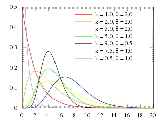
機率密度函式
累積分佈函式
引數	$\scriptstyle k\;>\;0$ 形狀 $\scriptstyle \theta \;>\;0\,$ 尺度
支援	$\scriptstyle x\;\in \;(0,\,\infty )\!$
PDF	$\scriptstyle {\frac {1}{\Gamma (k)\theta ^{k}}}x^{k\,-\,1}e^{-{\frac {x}{\theta }}}\,\!$
CDF	$\scriptstyle {\frac {1}{\Gamma (k)}}\gamma \left(k,\,{\frac {x}{\theta }}\right)\!$
均值	$\scriptstyle \operatorname {E} [X]=k\theta \!$ $\scriptstyle \operatorname {E} [\ln X]=\psi (k)+\ln(\theta )\!$ (參見雙伽馬函式)
中位數	沒有簡單的閉合形式
眾數	$\scriptstyle (k\,-\,1)\theta {\text{ for }}k\;>\;1\,\!$
方差	$\scriptstyle \operatorname {Var} [X]=k\theta ^{2}\,\!$ $\scriptstyle \operatorname {Var} [\ln X]=\psi _{1}(k)\!$ (參見三伽馬函式 )
偏度	$\scriptstyle {\frac {2}{\sqrt {k}}}\,\!$
例如峰度	$\scriptstyle {\frac {6}{k}}\,\!$
熵	$\scriptstyle {\begin{aligned}\scriptstyle k&\scriptstyle \,+\,\ln \theta \,+\,\ln[\Gamma (k)]\\\scriptstyle &\scriptstyle \,+\,(1\,-\,k)\psi (k)\end{aligned}}$

伽馬分佈在技術上非常重要，因為它指數分佈的母分佈，可以解釋許多其他分佈。

機率密度函式是

$f_{x}(x)={\begin{cases}{\frac {1}{a^{p}\Gamma (p)}}x^{p-1}e^{-x/a},&{\mbox{if }}x\geq 0\\0,&{\mbox{if }}x<0\end{cases}}\quad a,p>0$

其中 $\Gamma (p)=\int _{0}^{\infty }t^{p-1}e^{-t}\,dt\,$ 是伽馬函式。除非 p=1，否則累積分佈函式無法找到，在這種情況下，伽馬分佈將變為指數分佈。隨機變數 X 的伽馬分佈記為 $X\in \Gamma (p,a)$。

或者，伽馬分佈可以用形狀引數 $\alpha =k$ 和逆尺度引數 $\beta =1/\theta$，稱為速率引數，進行引數化

$g(x;\alpha ,\beta )=Kx^{\alpha -1}e^{-\beta \,x}\ \mathrm {for} \ x>0\,\!.$

其中，常數 $K$ 可以透過將密度函式的積分設定為 1 來計算

$\int _{-\infty }^{+\infty }g(x;\alpha ,\beta )\mathrm {d} t\,=\int _{0}^{+\infty }Kx^{\alpha -1}e^{-\beta \,x}\mathrm {d} x\,=1$

如下

$K\int _{0}^{+\infty }x^{\alpha -1}e^{-\beta \,x}\mathrm {d} x\,=1$

$K={\frac {1}{\int _{0}^{+\infty }x^{\alpha -1}e^{-\beta \,x}\mathrm {d} x}}$

並且，透過變數替換 $y=\beta x$ 

${\begin{aligned}K&={\frac {1}{\int _{0}^{+\infty }{\frac {y^{\alpha -1}}{\beta ^{\alpha -1}}}e^{-y}{\frac {\mathrm {d} y}{\beta }}}}\\&={\frac {1}{{\frac {1}{\beta ^{\alpha }}}\int _{0}^{+\infty }y^{\alpha -1}e^{-y}\mathrm {d} y}}\\&={\frac {\beta ^{\alpha }}{\int _{0}^{+\infty }y^{\alpha -1}e^{-y}\mathrm {d} y}}\\&={\frac {\beta ^{\alpha }}{\Gamma (\alpha )}}\end{aligned}}$

如下

$g(x;\alpha ,\beta )=x^{\alpha -1}{\frac {\beta ^{-\alpha }\,e^{-\beta \,x}}{\Gamma (\alpha )}}\ \mathrm {for} \ x>0\,\!.$

機率密度函式

我們首先檢查機率密度函式的總積分是否為 1。

$\int _{-\infty }^{\infty }{\frac {1}{a^{p}\Gamma (p)}}x^{p-1}e^{-x/a}dx$

現在我們令y=x/a，這意味著dy=dx/a

${\frac {1}{\Gamma (p)}}\int _{0}^{\infty }y^{p-1}e^{-y}dy$

${\frac {1}{\Gamma (p)}}\Gamma (p)=1$

均值

$\operatorname {E} [X]=\int _{-\infty }^{\infty }x\cdot {\frac {1}{a^{p}\Gamma (p)}}x^{p-1}e^{-x/a}dx$

現在我們令y=x/a，這意味著dy=dx/a。

$\operatorname {E} [X]=\int _{0}^{\infty }ay\cdot {\frac {1}{\Gamma (p)}}y^{p-1}e^{-y}dy$

$\operatorname {E} [X]={\frac {a}{\Gamma (p)}}\int _{0}^{\infty }y^{p}e^{-y}dy$

$\operatorname {E} [X]={\frac {a}{\Gamma (p)}}\Gamma (p+1)$

現在我們利用這個事實：$\Gamma (z+1)=z\Gamma (z)$

$\operatorname {E} [X]={\frac {a}{\Gamma (p)}}p\Gamma (p)=ap$

方差

我們首先計算E[X^2]

$\operatorname {E} [X^{2}]=\int _{-\infty }^{\infty }x^{2}\cdot {\frac {1}{a^{p}\Gamma (p)}}x^{p-1}e^{-x/a}dx$

現在我們令y=x/a，這意味著dy=dx/a。

$\operatorname {E} [X^{2}]=\int _{0}^{\infty }a^{2}y^{2}\cdot {\frac {1}{a\Gamma (p)}}y^{p-1}e^{-y}ady$

$\operatorname {E} [X^{2}]={\frac {a^{2}}{\Gamma (p)}}\int _{0}^{\infty }y^{p+1}e^{-y}dy$

$\operatorname {E} [X^{2}]={\frac {a^{2}}{\Gamma (p)}}\Gamma (p+2)=pa^{2}(p+1)$

現在我們計算方差

$\operatorname {Var} (X)=\operatorname {E} [X^{2}]-(\operatorname {E} [X])^{2}$

$\operatorname {Var} (X)=pa^{2}(p+1)-(ap)^{2}=pa^{2}$

外部連結

• 互動式伽馬分佈網路小程式（Java）