分形/複平面迭代/q迭代

透過臨界軌道逆迭代繪製的Julia集（在Siegel圓盤的情況下）

用向後迭代生成的動態平面的週期性外部射線

迭代在數學中指的是迭代一個函式的過程，即重複應用一個函式，使用一次迭代的輸出作為下一次迭代的輸入。 即使是看似簡單的函式的迭代也會產生複雜的行為和難題。

應用

可以進行逆（向後迭代）

• 排斥器用於繪製Julia集（IIM/J）
• Jlia集外的圓圈（半徑=ER）用於繪製逃逸時間等值線（趨向於Julia集）
• Julia集內的圓圈（半徑=AR）用於繪製吸引時間等值線（趨向於Julia集）
• 臨界軌道（在Siegel圓盤情況下）用於繪製Julia集（可能僅在黃金分割的情況下）
• 用於繪製外部射線

向前迭代的排斥器是向後迭代的吸引器

備註

• 迭代始終在動態平面上。
• 引數平面上沒有動態。
• Mandelbrot集沒有動力學。它是一組引數值。
• 引數平面上沒有軌道，不應該在引數平面上繪製軌道。
• 臨界點的軌道在動態平面上

迭代理論

這是安德魯·羅賓斯2006-02-15在Tetration論壇上的文章的一部分，作者是安德魯·羅賓斯

"迭代是動力學、混沌、分析、遞迴函式和數論的基礎。在這些學科中，大多數情況下所需的迭代是整數迭代，即迭代引數為整數。然而，在動力系統研究中，連續迭代對於解決某些系統至關重要。

不同的迭代型別可以分類如下

• 離散迭代
  • 整數迭代
  • 分數迭代或有理迭代
    • 非解析分數迭代
    • 解析分數迭代
• 連續迭代

離散迭代

迭代函式

• 例子
• 導數

整數迭代

迭代的通常定義，其中函式方程

$f^{n}(x)=f(f^{n-1}(x))$

用於生成序列

$\{f(x),f^{2}(x),f^{3}(x),...\}$

稱為f(x)的自然迭代，在組合下形成一個么半群。

對於可逆函式f(x)，逆函式也被認為是迭代，並形成序列

$\{...,f^{-2}(x),f^{-1}(x),x,f(x),f^{2}(x),...\}$

稱為f(x)的整數迭代，在組合下形成一個群。

分數迭代或有理迭代

求解函式方程：$f(x)=g^{n}(x)$。求解完該函式方程後，就可以求出有理迭代$f^{(m/n)}(x)$，即$g(x)$的整數迭代。

非解析分數迭代

選擇非解析分數迭代，得到的結果將不是唯一的。（Iga 的方法）

解析分數迭代

求解解析分數迭代，將得到一個唯一的解。（Dahl 的方法）

連續迭代

這是對通常迭代概念的推廣，其中函式方程（FE）：f n(x) = f(f n-1(x)) 必須在域（實數或複數）的所有 n 中成立。如果不是這樣，那麼為了討論這些型別的“迭代”（即使它們在技術上不是“迭代”，因為它們不遵循迭代的 FE），我們將討論它們，就好像它們是 f n(x) 的表示式，其中 0 ≤ Re(n) ≤ 1，並且在其他地方由迭代的 FE 定義。因此，即使一種方法是解析的，如果它不滿足這個基本的 FE，那麼根據這個重新定義，它就是非解析的。

非解析連續迭代

選擇非解析連續迭代，得到的結果將不是唯一的。（Galidakis 和 Woon 的方法）

解析連續迭代或解析迭代

求解解析連續迭代，將得到一個唯一的解。

步長

• 整數
• 分數
• 動態對映的連續迭代。 該連續迭代可以透過有限元方法進行離散化，然後在計算機上並行求解。

視覺化

• 摺疊
• 復幾何序列 由 Loo Kang Lawrence WEE 製作

分解

在復二次多項式的情況下，迭代過程中的移動是複數。它包含 2 個移動

• 角移動 = 旋轉（參見倍增對映）
• 徑向移動（參見外部和內部射線，不變曲線）
  • 落入目標集和吸引子（在雙曲和拋物線情況下）

• 徑向移動
• 
  半徑 abs(z) = r < 1.0，經過一些使用 f0(z) = z*z 的迭代後
• 
  點的重複迭代之間的距離小於 1

• 角移動
• 
  倍增對映後的角度為 1/7
• 
  倍增對映後的角度為 1/15
• 
  倍增對映後的角度為 11/36

角移動（旋轉）

以轉數計算複數的幅角

/*
gives argument of complex number in turns 


*/

double GiveTurn( double complex z){
double t;

  t =  carg(z);
  t /= 2*pi; // now in turns
  if (t<0.0) t += 1.0; // map from (-1/2,1/2] to [0, 1) 
  return (t);
}

方向

反向

多值複數平方根函式的實部和虛部之間的過渡

反向迭代或逆迭代

• Peitgen
• W Jung
• John Bonobo

Peitgen

 /* Zn*Zn=Z(n+1)-c */
                Zx=Zx-Cx;
                Zy=Zy-Cy;
                /* sqrt of complex number algorithm from Peitgen, Jurgens, Saupe: Fractals for the classroom */
                if (Zx>0)
                {
                 NewZx=sqrt((Zx+sqrt(Zx*Zx+Zy*Zy))/2);
                 NewZy=Zy/(2*NewZx);        
                 }
                 else /* ZX <= 0 */
                 {
                  if (Zx<0)
                     {
                      NewZy=sign(Zy)*sqrt((-Zx+sqrt(Zx*Zx+Zy*Zy))/2);
                      NewZx=Zy/(2*NewZy);        
                      }
                      else /* Zx=0 */
                      {
                       NewZx=sqrt(fabs(Zy)/2);
                       if (NewZx>0) NewZy=Zy/(2*NewZx);
                          else NewZy=0;    
                      }
                 };
              if (rand()<(RAND_MAX/2))
              {   
                  Zx=NewZx;
                  Zy=NewZy; 
                  }
              else {Zx=-NewZx;
                  Zy=-NewZy; }

Mandel

以下是使用來自 Wolf Jung 編寫的程式 Mandel 的程式碼，進行逆迭代的 c 程式碼示例。

/*
/*

 gcc i.c -lm -Wall
 ./a.out
 
 
 
 
z = 0.000000000000000  +0.000000000000000 i
z = -0.229955135116281  -0.141357981605006 i
z = -0.378328716195789  -0.041691618297441 i
z = -0.414752103217922  +0.051390827017207 i



 


*/

#include <stdio.h>
#include <math.h> // M_PI; needs -lm also 
#include <complex.h>

/* find c in component of Mandelbrot set 
 
   uses code by Wolf Jung from program Mandel
   see function mndlbrot::bifurcate from mandelbrot.cpp
   http://www.mndynamics.com/indexp.html

*/
double complex GiveC(double InternalAngleInTurns, double InternalRadius, unsigned int Period)
{
  //0 <= InternalRay<= 1
  //0 <= InternalAngleInTurns <=1
  double t = InternalAngleInTurns *2*M_PI; // from turns to radians
  double R2 = InternalRadius * InternalRadius;
  double Cx, Cy; /* C = Cx+Cy*i */

  switch ( Period ) // of component 
    {
    case 1: // main cardioid
      Cx = (cos(t)*InternalRadius)/2-(cos(2*t)*R2)/4; 
      Cy = (sin(t)*InternalRadius)/2-(sin(2*t)*R2)/4; 
      break;
    case 2: // only one component 
      Cx = InternalRadius * 0.25*cos(t) - 1.0;
      Cy = InternalRadius * 0.25*sin(t); 
      break;
      // for each iPeriodChild  there are 2^(iPeriodChild-1) roots. 
    default: // higher periods : to do, use newton method 
      Cx = 0.0;
      Cy = 0.0; 
      break; }

  return Cx + Cy*I;
}

/* mndyncxmics::root from mndyncxmo.cpp  by Wolf Jung (C) 2007-2014. */

// input = x,y
// output = u+v*I = sqrt(x+y*i) 
complex double GiveRoot(complex double z)
{  
  double x = creal(z);
  double y = cimag(z);
  double u, v;
  
   v  = sqrt(x*x + y*y);

   if (x > 0.0)
        { u = sqrt(0.5*(v + x)); v = 0.5*y/u; return  u+v*I; }
   if (x < 0.0)
         { v = sqrt(0.5*(v - x)); if (y < 0.0) v = -v; u = 0.5*y/v; return  u+v*I; }
   if (y >= 0.0) 
       { u = sqrt(0.5*y); v = u; return  u+v*I; }

   u = sqrt(-0.5*y); 
   v = -u;
   return  u+v*I;
}

// from mndlbrot.cpp  by Wolf Jung (C) 2007-2014. part of Madel 5.12 
// input : c, z , mode
// c = cx+cy*i where cx and cy are global variables defined in mndynamo.h
// z = x+y*i
// 
// output : z = x+y*i
complex double InverseIteration(complex double z, complex double c, char key)
{
    double x = creal(z);
    double y = cimag(z);
    double cx = creal(c);
    double cy = cimag(c);
   
   // f^{-1}(z) = inverse with principal value
   if (cx*cx + cy*cy < 1e-20) 
   {  
      z = GiveRoot(x - cx + (y - cy)*I); // 2-nd inverse function = key b 
      if (key == 'B') { x = -x; y = -y; } // 1-st inverse function = key a   
      return -z;
   }
    
   //f^{-1}(z) =  inverse with argument adjusted
   double u, v;
   complex double uv ;
   double w = cx*cx + cy*cy;
    
   uv = GiveRoot(-cx/w -(cy/w)*I); 
   u = creal(uv);
   v = cimag(uv);
   //
   z =  GiveRoot(w - cx*x - cy*y + (cy*x - cx*y)*I);
   x = creal(z);
   y = cimag(z);
   //
   w = u*x - v*y; 
   y = u*y + v*x; 
   x = w;
  
   if (key =='A'){
    x = -x; 
    y = -y;  // 1-st inverse function = key a
  }
  return x+y*I; // key b =  2-nd inverse function

}


 /*f^{-1}(z) =  inverse with argument adjusted
    "When you write the real and imaginary parts in the formulas as complex numbers again,
       you see that it is sqrt( -c / |c|^2 )  *  sqrt( |c|^2 - conj(c)*z ) ,
     so this is just sqrt( z - c )  except for the overall sign:
    the standard square-root takes values in the right halfplane,  but this is rotated by the squareroot of -c .
    The new line between the two planes has half the argument of -c .
    (It is not orthogonal to c ...  )" 
    ...
    "the argument adjusting in the inverse branch has nothing to do with computing external arguments.  It is related to itineraries and kneading sequences,  ...
    Kneading sequences are explained in demo 4 or 5, in my slides on the stripping algorithm, and in several papers by Bruin and Schleicher.
 
    W Jung " */
    
    
double complex GiveInverseAdjusted (complex double z, complex double c, char key){

  
  double t = cabs(c);
  t = t*t;
  
  
  z =  csqrt(-c/t)*csqrt(t-z*conj(c)); 
  if (key =='A') z = -z; // 1-st inverse function = key a
  // else key == 'B'
  return z; 


}   








// make iMax inverse iteration with negative sign ( a in Wolf Jung notation )
complex double GivePrecriticalA(complex double z, complex double c, int iMax)
{
  complex double za = z;  
  int i; 
  
  
  for(i=0;i<iMax ;++i){
    printf("i = %d ,  z = (%f, %f) \n ", i,  creal(za), cimag(za) );
    za = InverseIteration(za,c, 'A'); 
    

   }

 printf("i = %d ,  z = (%f, %f) \n ", i,  creal(za), cimag(za) );
 return za;
}



// make iMax inverse iteration with negative sign ( a in Wolf Jung notation )
complex double GivePrecriticalA2(complex double z, complex double c, int iMax)
{
  complex double za = z;  
  int i; 
  
  
  for(i=0;i<iMax ;++i){
    printf("i = %d ,  z = (%f, %f) \n ", i,  creal(za), cimag(za) );
    za = GiveInverseAdjusted(za,c, 'A'); 
    

   }

 printf("i = %d ,  z = (%f, %f) \n ", i,  creal(za), cimag(za) );
 return za;
}





int main(){
  
 complex double c;
 complex double z;
 complex double zcr = 0.0; // critical point

 int iMax = 10;
 int iPeriodChild = 3; // period of
 int iPeriodParent = 1;

 
     c = GiveC(1.0/((double) iPeriodChild), 1.0, iPeriodParent); // root point = The unique point on the boundary of a mu-atom of period P where two external angles of denominator = (2^P-1) meet.
     z = GivePrecriticalA( zcr, c, iMax);
     printf("iAngle = %d/%d  c = (%f, %f); z = (%.16f, %.16f) \n ", iPeriodParent,  iPeriodChild, creal(c), cimag(c), creal(z), cimag(z) );

      z = GivePrecriticalA2( zcr, c, iMax);
     printf("iAngle = %d/%d  c = (%f, %f); z = (%.16f, %.16f) \n ", iPeriodParent,  iPeriodChild, creal(c), cimag(c), creal(z), cimag(z) );

return 0; 
}

測試

可以無限次迭代。測試將告知何時可以停止。

• 正向迭代的逃逸測試

目標集或陷阱

目標集 用於測試。當 zn 在目標集中時，就可以停止迭代。

平面

引數平面

"曼德布羅特集沒有動力學。它是一組引數值。引數平面上沒有軌道，不應該在引數平面上繪製軌道。臨界點的軌道在動力學平面上"

動態平面

  "The polynomial Pc maps each dynamical ray to another ray doubling the angle (which we measure in full turns, i.e. 0 = 1 = 2π rad = 360◦), and the dynamical rays of any polynomial “look like straight rays” near infinity. This allows us to study the
   Mandelbrot and Julia sets combinatorially, replacing the dynamical plane by the unit circle, rays by angles, and the quadratic polynomial by the doubling modulo one map." Virpi K a u k o

c=0時的動態平面 f0

具有勢函式 $\phi (x,y)={\sqrt {x^{2}+y^{2}}}$ 的徑向向量場的等勢曲線（紅色）和積分曲線（藍色）。

假設 c=0，那麼可以將動力學平面稱為 $f_{0}$ 平面。

這裡，動力學平面可以被分為：

• Julia 集 = $\{z:|z|=1\}$
• Fatou 集，它包含兩個子集：
  • Julia 集的內部 = 有限吸引子的吸引域 = $\{z:|z|<1\}$
  • Julia 集的外部 = 無窮大的吸引域 = $\{z:|z|>1\}$

正向迭代

單位圓內的複數的 10 次方

指數螺旋

arg 的主值分支

$z=re^{i\theta }\,$

其中：

• r 是複數 z = x + i 的絕對值、模數 或幅值
• $\theta$ 是複數 z 的輻角（在許多應用中稱為“相位”），是半徑與正實軸的夾角。通常使用主值。

$r=|z|={\sqrt {x^{2}+y^{2}}}.\,$

$\theta =\arg(z)=\operatorname {atan2} (y,x)={\begin{cases}\arctan({\frac {y}{x}})&{\mbox{if }}x>0\\\arctan({\frac {y}{x}})+\pi &{\mbox{if }}x<0{\mbox{ and }}y\geq 0\\\arctan({\frac {y}{x}})-\pi &{\mbox{if }}x<0{\mbox{ and }}y<0\\{\frac {\pi }{2}}&{\mbox{if }}x=0{\mbox{ and }}y>0\\-{\frac {\pi }{2}}&{\mbox{if }}x=0{\mbox{ and }}y<0\\{\mbox{indeterminate }}&{\mbox{if }}x=0{\mbox{ and }}y=0.\end{cases}}$

因此

$f_{0}(z)=z^{2}=(re^{i\theta })^{2}=r^{2}e^{i2\theta }\,$

以及前向迭代：

$f_{0}^{n}(z)=r^{2^{n}}e^{i2^{n}\theta }\,$

正向迭代

• 對半徑平方並使角度翻倍（相位，幅角）
• 得到前向軌跡 = **點列表** {z0, z1, z2, z3... , zn}，這些點位於指數螺旋線上。

你可以互動式地檢查它

• Geogebra plet by Jorj Kowszun-Lecturer - 嘗試沿著從中心到外邊的徑向線移動，看看行為的變化
• M McClure 對複數平方迭代的視覺化
• W Jung 的 Mandel 程式
• Jeffrey Ventrella 對複數的平方
• MIT mathlets：複數指數

混沌與複數平方對映

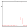
迭代呈現混沌現象的非正式原因是，角度在每次迭代中翻倍，而翻倍隨著角度變得越來越大而迅速增長，但相差 2π 弧度的倍數的角度是相同的。因此，當角度超過 2π 時，它必須透過 2π 除以餘數進行*迴圈*。因此，角度根據二元變換（也稱為 2x 模 1 對映）進行變換。由於初始值 *z*₀ 被選擇為其幅角不是 π 的有理倍數，因此 *z*_*n* 的前向軌跡不能重複自身並變得週期性。

更正式地說，迭代可以寫成

$\qquad z_{n+1}=z_{n}^{2}$

其中 $z_{n}$ 是透過迭代上述步驟獲得的複數序列，而 $z_{0}$ 代表初始起始數字。我們可以精確地解決此迭代

$\qquad z_{n}=z_{0}^{2^{n}}$

從角度 θ 開始，我們可以將初始項寫成 $z_{0}=\exp(i\theta )$，因此 $z_{n}=\exp(i2^{n}\theta )$。這使得角度的連續加倍變得清晰。（這等效於關係 $z_{n}=\cos(2^{n}\theta )+i\sin(2^{n}\theta )$）。

逃逸測試

如果距離

• 點 z 屬於 Julia 集外部
• Julia 集 $J_{c}$

是

$distance(z,J_{c})=2^{-n}$

那麼點 z 逃逸（= 它的幅度大於 逃逸半徑 = ER）

$|z_{n}|>ER$

之後

• $n$ 步在非拋物線情況下
• $2^{n}$ 步在 拋物線情況下

另請參閱

• 逃逸測試所需的精度
• 逃逸測試
• 逃逸時間
• david bau：複函式檢視器

反向迭代

使用適當選擇的原像對復二次多項式進行反向迭代

每個角度（實數）α ∈ R/Z 以周為單位測量，都具有

• 一個像 = 2α mod 1 在 倍增對映 下
• "在 倍增對映 下有兩個原像：${\frac {\alpha }{2}},{\frac {\alpha +1}{2}}$”。 倍增對映的逆函式是多值函式。

注意，這兩個原像之間的差異

${\frac {\alpha }{2}}-{\frac {\alpha +1}{2}}={\frac {1}{2}}$

是半個週轉 = 180 度 = Pi 弧度。

在倍增對映 d 下的像和原像

$\alpha$	$d^{1}(\alpha )$	$d^{-1}(\alpha )$
${\frac {1}{2}}$	${\frac {1}{1}}$	$\left\{{\frac {1}{4}},{\frac {3}{4}}\right\}$
${\frac {1}{3}}$	${\frac {2}{3}}$	$\left\{{\frac {1}{6}},{\frac {4}{6}}\right\}$
${\frac {1}{4}}$	${\frac {1}{2}}$	$\left\{{\frac {1}{8}},{\frac {5}{8}}\right\}$
${\frac {1}{5}}$	${\frac {2}{5}}$	$\left\{{\frac {1}{10}},{\frac {6}{10}}\right\}$
${\frac {1}{6}}$	${\frac {1}{3}}$	$\left\{{\frac {1}{12}},{\frac {7}{12}}\right\}$
${\frac {1}{7}}$	${\frac {2}{7}}$	$\left\{{\frac {1}{14}},{\frac {4}{7}}\right\}$

在復動力平面使用二次多項式 $f_{c}$ 進行反向迭代

$f_{c}(z)=z^{2}+c$

給出反向軌道 = **原像的二叉樹** 

$z\,$

$-{\sqrt {z-c}},+{\sqrt {z-c}}\,$

$-{\sqrt {-{\sqrt {z-c}}-c}},+{\sqrt {-{\sqrt {z-c}}-c}},-{\sqrt {+{\sqrt {z-c}}-c}},+{\sqrt {+{\sqrt {z-c}}-c}}\,$

在這樣的樹中，如果沒有額外資訊，就無法選擇好的路徑。

注意，原象顯示旋轉對稱性（180 度）

有關其他函式，請參閱 Fractalforum

另請參閱

• 史蒂夫·菲爾普斯繪製的朱莉婭集網格。z=sqrt(z-c) 對映在 Geogebra 上

fc 的動態平面

可以使用以下方法進行檢查

• M McClure：視覺化：互動式盆地
• 馬克·達布斯製作的 GeoGebra - 複雜迭代 - 曼德勃羅集
• 傑里米·裡夫金繪製的臨界軌道

逃逸時間或吸引時間的等高線

• 
  外部圓的原象給出逃逸時間的等高線
• 
  內部圓的原象給出吸引時間的等高線

IIM/J 繪製的朱莉婭集

理論

• 週期點在朱莉婭集中稠密
• 朱莉婭集是排斥週期點的集合的閉包

因此，繪製排斥週期點及其軌道（正向和反向 = 逆向）可以直觀地很好地近似朱莉婭集 = 點集足夠稠密，這些點在朱莉婭集上的非均勻分佈並不重要。

• 
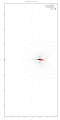
  當 C = i 時，排斥不動點的原象趨向於朱莉婭集。影像和原始碼
• 
  使用 MIIM 繪製的朱莉婭集。影像和 Maxima 原始碼
• 
  在西格爾圓盤情況下，臨界軌道的原象趨向於整個朱莉婭集
• 
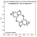
  簡單 IIM/J 中的點分佈
• 
  c = -0.750357820200574 +0.047756163825227 i
• 
  C = ( 0.4 0.3 )

在逃逸時間中，計算點 z 的正向迭代。

在 IIM/J 中，計算

• 複雜二次多項式的排斥不動點 $Z_{0}=\beta _{c}\,$
• 透過逆向迭代計算 $Z_{0}\,$ 的原象

$Z_{n-1}={\sqrt {Z_{n}-C}}$

 "We know the periodic points are dense in the Julia set, but in the case of weird ones (like the ones with Cremer points, or even some with Siegel disks where the disk itself is very 'deep' within the Julia set, as measured by the external rays), the periodic points tend to avoid certain parts of the Julia set as long as possible. This is what causes the 'inverse method' of rendering images of Julia sets to be so bad for those cases." Jacques Carette

因為平方根是多值函式，所以每個 $Z_{n}\,$ 都有兩個原象 $Z_{n-1}\,$。因此，逆向迭代會建立二叉樹 的原象。

• 
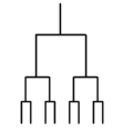  二叉樹
• 
  二叉樹的擴充套件增長

由於二叉樹的擴充套件增長，原象的數量呈指數級增長：完整二叉樹中節點的數量 $n$ 為

$n=2^{h+1}-1$

其中

• $h$ 是樹的高度

如果要繪製完整二叉樹，則儲存二叉樹的方法會浪費大量記憶體，因此另一種方法是

• 執行緒二叉樹
• 只繪製二叉樹中的某些路徑
  • 隨機路徑：最長路徑 = 從根到葉的路徑

另請參閱

• 線上工具：Wolfram Alpha

樹的根

• 複雜二次多項式的排斥不動點 $Z_{0}=\beta _{c}\,$
• - beta
• 其他排斥週期點（填充的朱利亞集的切割點）。這在拋物線朱利亞集的情況下尤其重要。

“...排斥不動點β的原像。它們形成一棵樹狀的

                                               beta
                    beta                                            -beta
   beta                         -beta                    x                     y

因此，當您從β開始構建樹時，每個點最終都會被計算兩次。如果您從-β開始，您將獲得相同數量的點，但計算次數減半。

類似的情況也適用於臨界軌道的原像。如果z在臨界軌道上，它的兩個原像中也會有一個在其中，所以您應該繪製-z及其原像的樹，以避免重複計算相同點。”（Wolf Jung）

IIM 的變體

• 隨機選擇兩個根中的一個 IIM（直到選擇的最大級別）。隨機遍歷樹。最簡單的編碼和快速，但效率低下。從它開始。
  • 兩個根以相同的機率
  • 一個根比另一個根更頻繁
• 繪製所有根（直到選擇的最大級別）
  • 使用遞迴
  • 使用堆疊（更快？）
• 在二叉樹中繪製一些罕見路徑 = MIIM。這是繪製所有根的修改。停止使用一些罕見路徑。
  • 使用命中表（while hit(pixel(iX,iY)) < HitMax）
  • 使用導數（while derivative(z) < DerivativeMax）
    • “透過修剪樹的密集分支來加快計算速度。一種這樣的方法是在對映變得收縮（累積導數變大）時修剪分支。”Paul Nylander
    • “如果導數大於極限，我們就從給定的位置切斷子樹。這消除了逆迭代中占主導地位的、高度收縮的區域，這些區域已經被記錄下來。我們可以迭代地計算後續的導數。用絕對導數的對數來著色”

程式碼示例

與之比較

• C 程式碼.
• Matlab 程式碼

另請參閱

• 顏色：朱利亞集的不同部分具有不同的顏色
  • 虛擬數學博物館：朱利亞集
  • fractalforums.org：朱利亞集

另請參閱

• 動力系統
  • 不動點
  • 李雅普諾夫數
• 函式方程
  • 阿貝爾函式
  • 施羅德函式
  • 博特切函式
  • 朱利亞函式
• 特殊矩陣
  • 卡萊曼矩陣
  • 貝爾矩陣
  • 阿貝爾-羅賓斯矩陣