   "... a single algorithm for computing all quadratic Julia sets does not exist."^[1]

本書展示瞭如何為在動態平面中繪製集合編寫不同的演算法：Julia、填充的 Julia 或 Fatou 集，用於復二次多項式。它分為兩部分

各種演算法的描述^[2]
動態平面中各種集合視覺化技術的描述
- Julia 集
- Fatou 集
  - 無限吸引盆 (開集)
  - 有限吸引子的吸引盆

演算法

基於吸引速度的方法

這裡顏色與吸引速度 (收斂到吸引子) 成正比。這些方法用於 Fatou 集。

如何找到

最低最優逃逸值 (IterationMax)？^[3]
逃逸半徑^[4]

無限吸引盆 = 填充的 Julia 集外部和發散方案 = 逃逸時間方法 (ETM)

首先閱讀定義

這裡計算復點 Z₀ 的正向迭代

$Z_{n+1}=Z_{n}^{2}+C$

這是一個計算最後迭代的函式，即第一個落在目標集中的迭代 (例如，離開以給定逃逸半徑 ER 為中心的圓) 用於上述復二次多項式的迭代。這是一個迭代 (整數)，對於它 (abs(Z)>ER) 成立。它也可以改進^[5]

C 版本 (這裡 ER2=ER*ER) 使用雙精度浮點數 (沒有複數型別數字)

 int GiveLastIteration(double Zx, double Zy, double Cx, double Cy, int IterationMax, int ER2)
 {
  double Zx2, Zy2; /* Zx2=Zx*Zx;  Zy2=Zy*Zy  */
  int i=0;
  Zx2=Zx*Zx;
  Zy2=Zy*Zy;
  while (i<IterationMax && (Zx2+Zy2<ER2) ) /* ER2=ER*ER */
  {
   Zy=2*Zx*Zy + Cy;
   Zx=Zx2-Zy2 +Cx;
   Zx2=Zx*Zx;
   Zy2=Zy*Zy;
   i+=1;
  }
  return i;
 }

帶有來自 GSL 的複數型別的 C：^[6]

#include <gsl/gsl_complex.h>
#include <gsl/gsl_complex_math.h>
#include <stdio.h>
// gcc -L/usr/lib -lgsl -lgslcblas -lm t.c 
// function fc(z) = z*z+c

gsl_complex f(gsl_complex z, gsl_complex c) {
  return gsl_complex_add(c, gsl_complex_mul(z,z));
}

int main () {
  gsl_complex c = gsl_complex_rect(0.123, 0.125);
  gsl_complex z = gsl_complex_rect(0.0, 0.0);
  int i;
  for (i = 0; i < 10; i++) {
    z = f(z, c);
    double zx = GSL_REAL(z);
    double zy = GSL_IMAG(z);
    printf("Real: %f4 Imag: %f4\n", zx, zy);
  }
  return 0;
}

C++ 版本:

 int GiveLastIteration(complex C,complex Z , int imax, int ER)
  {
   int i; // iteration number
   for(i=0;i<=imax-1;i++) // forward iteration
    {
      Z=Z*Z+C; // overloading of operators
      if(abs(Z)>ER) break;
    }
   return i;
 }

#include <complex> // C++ complex library

// bailout2 = bailout * bailout
// this function is based on function esctime from mndlbrot.cpp 
// from program mandel ver. 5.3 by Wolf Jung
// http://www.mndynamics.com/indexp.html

int escape_time(complex<double> Z, complex<double> C , int iter_max,  double bailout2)
{ 
  // z= x+ y*i   z0=0
  long double x =Z.real(), y =Z.imag(),  u ,  v ;
  int iter; // iteration
  for ( iter = 0; iter <= iter_max-1; iter++)
  { u = x*x; 
    v = y*y;
    if ( u + v <= bailout2 ) 
       { 
         y = 2 * x * y + C.imag();
         x = u - v + C.real(); 
       } // if
    else break;
  } // for 
  return iter;
} // escape_time

^[7]

Delphi 版本 (使用使用者定義的複數型別、cabs 和 f 函式)

function GiveLastIteration(z,c:Complex;ER:real;iMax:integer):integer;
  var i:integer;
  begin
  i:=0;
  while (cabs(z)<ER) and (i<iMax) do
    begin
      z:= f(z,c);
      inc(i);
    end;
  result := i;
end;

其中

type complex = record x, y: real; end;

function cabs(z:complex):real;
begin
  cabs:=sqrt(z.x*z.x+z.y*z.y)
end;

function f(z,c:complex):complex; // complex quadratic polynomial
  var tmp:complex;
begin
  tmp.x := (z.x*z.x) - (z.y*z.y) + c.x;
  tmp.y := 2*z.x*z.y + c.y ;
  result := tmp;

end;

沒有明確定義複數的 Delphi 版本

function GiveLastIteration(zx0,zy0,cx,cy,ER2:extended;iMax:integer):integer;
  // iteration of z=zx+zy*i under fc(z)=z*z+c
  // where c=cx+cy*i
  // until abs(z)<ER  ( ER2=ER*ER )  or i>=iMax
  var i:integer;
      zx,zy,
      zx2,zy2:extended;
  begin
  zx:=zx0;
  zy:=zy0;
  zx2:=zx*zx;
  zy2:=zy*zy;

  i:=0;
  while (zx2+zy2<ER2) and (i<iMax) do
    begin
      zy:=2*zx*zy + cy;
      zx:=zx2-zy2 +cx;
      zx2:=zx*zx;
      zy2:=zy*zy;
      //
      inc(i);
    end;
  result := i;
end;

Euler 版本 由 R. Grothmann 編寫 (略微更改：從 z^2-c 到 z^2+c) ^[8]

function iter (z,c,n=100) ...

h=z;
loop 1 to n;
h=h^2 + c;
if totalmax(abs(h))>1e20; m=#; break; endif;
end;
return {h,m};
endfunction

Lisp 版本

此版本使用複數。它使程式碼變短，但效率也很低。

((DEFUN GIVELASTITERATION (Z_0 _C IMAX ESCAPE_RADIUS) 
  (SETQ Z Z_0) 
  (SETQ I 0)
  (LOOP WHILE (AND (< I IMAX) (< (ABS Z) ESCAPE_RADIUS)) DO 
    (INCF I)
    (SETQ Z (+ (* Z Z) _C)))
   I)

Maxima 版本

/* easy to read but very slow version, uses complex type numbers */ 
GiveLastIteration(z,c):=
 block([i:0],
  while abs(z)<ER and i<iMax
     do (z:z*z + c,i:i+1),
  i)$

/* faster version, without use of complex type numbers,
   compare with c version, ER2=ER*ER */  
GiveLastIter(zx,zy,cx,cy,ER2,iMax):=
block(
 [i:0,zx2,zy2],
 zx2:zx*zx,
 zy2:zy*zy,
 while (zx2+zy2<ER2) and i<iMax do
 (	
  zy:2*zx*zy + cy,
  zx:zx2-zy2 +cx,
  zx2:zx*zx,
  zy2:zy*zy,
  i:i+1
 ),
 return(i)
);

布林逃逸時間

演算法：對於動態平面 (z 平面) 的每個點 z，計算 z 的幅度大於逃逸半徑的迭代次數 (最後迭代)。如果 last_iteration=max_iteration，則該點位於填充的 Julia 集中，否則它位於其補集 (無限的吸引盆) 中。這裡有兩個選項，因此它被稱為布林演算法。

if (LastIteration==IterationMax)
   then color=BLACK;   /* bounded orbits = Filled-in Julia set */
   else color=WHITE;  /* unbounded orbits = exterior of Filled-in Julia set  */

理論上，該方法用於繪製填充的 Julia 集及其補集 (外部)，但當 c 是 Misiurewicz 點 ( 填充的 Julia 集沒有內部) 時，該方法不會繪製任何東西。例如對於 c=i。這意味著它非常適合繪製填充的 Julia 集的內部。

ASCII 圖形

; common lisp
(loop for y from -2 to 2 by 0.05 do
      (loop for x from -2 to 2 by 0.025 do
		(let* ((z (complex x y))
                   	(c (complex -1 0))
                   	(iMax 20)
			(i 0))

		(loop  	while (< i iMax ) do 
			(setq z (+ (* z z) c))
			(incf i)
			(when (> (abs z) 2) (return i)))
			

           (if (= i iMax) (princ (code-char 42)) (princ (code-char 32)))))
      (format t "~%"))

帶有光柵圖形的 PPM 檔案

整數逃逸時間 = 無限吸引盆的水平集 = 水平集方法 = LSM/J

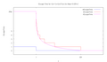
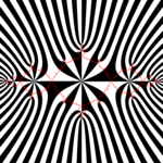
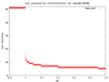C=0 且 0.9<Z<1.5 時逃逸時間的水平集

逃逸時間測量逃逸到無窮大的時間（無窮大是多項式的超吸引點）。時間以逃逸出給定半徑圓圈所需的步數（迭代 = i）來衡量（ER = 逃逸半徑）。

你可以看到一些東西

這是一個不連續函式
對於填充的 Julia 集中的 z，i 等於 iMax
對於 x0>ER，i=0
這是一個非線性函式

這裡的水平集是具有相同逃逸時間的點集。以下是黑白版本中選擇顏色的演算法。

  if (LastIteration==IterationMax)
   then color=BLACK;   /* bounded orbits = Filled-in Julia set */
   else   /* unbounded orbits = exterior of Filled-in Julia set  */
        if ((LastIteration%2)==0) /* odd number */
           then color=BLACK; 
           else color=WHITE;

以下是 c 函式，它

使用複數雙精度型別
計算 8 位顏色（灰度色調）
檢查逃逸和吸引測試

unsigned char ComputeColorOfLSM(complex double z){

 int nMax = 255;
  double cabsz;
  unsigned char iColor;
	
  int n;

  for (n=0; n < nMax; n++){ //forward iteration
	cabsz = cabs(z);
    	if (cabsz > ER) break; // esacping
    	if (cabsz< PixelWidth) break; // fails into finite attractor = interior
  			
   
     	z = z*z +c ; /* forward iteration : complex quadratic polynomial */ 
  }
  
  
  iColor = 255 - 255.0 * ((double) n)/20; // nMax or lower walues in denominator
  
  
  return iColor;
}

 "if a 2-variable function z = f(x,y) has non-extremal critical points, i.e. it has saddle points, then it's best if the contour z heights are chosen so that the saddle points are on a contour, so that the crossing contours appear visually."Alan Ableson

如何選擇水平曲線穿過臨界點（及其前像）的引數？

選擇引數 c 使其位於逃逸線上，那麼臨界值也將位於逃逸線上
選擇逃逸半徑等於臨界值的第 n 次迭代

// find such ER for LSM/J that level curves croses critical point and it's preimages ( only for disconnected Julia sets)
double GiveER(int i_Max){

	complex double z= 0.0; // criical point
	int i;
	 ; // critical point escapes very fast here. Higher valus gives infinity
	for (i=0; i< i_Max; ++i ){
		z=z*z +c; 
	 
	 }
	 
	 return cabs(z);
	
	
}

水平曲線在臨界點處交叉
不交叉
交叉
交叉

歸一化迭代次數（真實逃逸時間或分數迭代或平滑迭代計數演算法 (SICA)）

整數逃逸時間 = LSM
真實逃逸時間
C=0 且 0.5<Z<2.5 時的逃逸時間

數學公式

\nu (z)=\lim \limits _{i\to \infty }(i-\log _{2}\log _{2}|z_{i}|)\ .

Maxima 版本

GiveNormalizedIteration(z,c,E_R,i_Max):=
/* */
block(
 [i:0,r],
 while abs(z)<E_R and i<i_Max
   do (z:z*z + c,i:i+1),
 r:i-log2(log2(cabs(z))),
 return(float(r))
)$

在 Maxima 中，log(x) 是 x 的自然（以 e 為底）對數。要計算 log2，請使用

log2(x) := log(x) / log(2);

描述

逃逸時間水平曲線方法 = eLCM/J

邊緣檢測影像和 C 程式碼
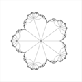
圓的前像

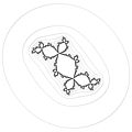
這些曲線是逃逸時間水平集的邊界（eLSM/J）。它們可以使用以下方法繪製

水平曲線的邊緣檢測（= 水平集的邊界）。
- 基於 M. Romera 等人的論文的演算法^[9]
- 索貝爾濾波器
繪製勒尼薩卡 = 曲線 $L_{n}=\{z:abs(z_{n})=ER\}\,$ ，參見解釋和原始碼
繪製圓圈 $L_{0}=\{z:abs(z)=ER\}\,$ 及其前像。參見此影像、解釋和原始碼
Harold V. McIntosh 描述的方法^[10]

/* Maxima code : draws lemniscates of Julia set */
c: 1*%i;
ER:2;
z:x+y*%i;
f[n](z) := if n=0 then z else (f[n-1](z)^2 + c);
load(implicit_plot); /* package by Andrej Vodopivec */ 
ip_grid:[100,100];
ip_grid_in:[15,15];
implicit_plot(makelist(abs(ev(f[n](z)))=ER,n,1,4),[x,-2.5,2.5],[y,-2.5,2.5]);

水平曲線的密度^[11]

  "The spacing between level curves is a good way to estimate gradients: level curves that are close together represent areas of steeper descent/ascent." ^[12]

 "The density of the contour lines tells how steep is the slope of the terrain/function variation. When very close together it means f is varying rapidly (the elevation increase or decrease rapidly). When the curves are far from each other the variation is slower" ^[13]

如何控制水平曲線

逃逸半徑
目標集的形狀
手動
- 繪製等勢線
- 更改水平集（水平曲線是水平集的邊界）

有限吸引子的吸引盆 = 填充的 Julia 集的內部

如何找到週期吸引子？
到達吸引子需要多少迭代？

填充的 Julia 集內部的組成部分（法圖集）

使用有限顏色（調色盤 = 編號顏色的列表）
找到吸引迴圈的週期
找到吸引迴圈的一個點
計算點到達吸引子後的迭代次數
元件的顏色 = 迭代 % 週期^[14]
使用邊緣檢測繪製 Julia 集

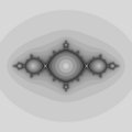
週期為 4 的法圖集的組成部分
週期為 3 的法圖集的組成部分
在西格爾盤的情況下，臨界軌道是邊界西格爾盤組成部分。所有其他組成部分都是該組成部分的前像

內部水平集

參見

Wolf Jung 編寫的 Mandel 程式的演算法 0

吸引
吸引
吸引
拋物線型
沿內部射線 0 的 c 的影片
弱吸引
拋物線型週期 3

如何選擇吸引陷阱的大小，使水平曲線在臨界點處交叉？

這取決於

動態型別（超吸引/吸引、拋物線型、排斥型）
週期（拋物線型情況下的子週期）

拋物線型情況下的花瓣
- 對於週期 1 和 2：以拋物點為中心的圓形，拋物點位於圓形邊界上
- 對於更高的週期，以拋物點為中心的圓形扇區
對於其他情況（除了排斥），它是以吸引子為中心的圓形半徑

int local_setup(double cx){
	
	c = cx;
	zp = GiveFixed(c);
	
	switch ( DynamicType){
		case repelling: // no  interior = no attracting fixed point = only escaping points
				
			break;
		case attracting: 
			delta = sqrt(1.0 - 4.0* creal(c));  // delta is a distance between alfa and beta fixed points
			AR =  delta /20.0;
			
	  		break;
  			
		case superattracting: // cabs(zp - zcr_last ) < PixelWidth 
			AR = 30.0* PixelWidth * iWidth / 5000 ; // 
	  		break;
		
		case parabolic:
				// zcr_last < parabolic_trap_center < zp
				int i; /* nr of point of critical orbit */
  				complex double z = zcr;
  				for (i=1;i<IterMax ; ++i) 
    					{ z = f(z); }
  				zcr_last = z;
				//
				AR = (zp - zcr_last)/2.0;
				parabolic_trap_center = ( creal(zp) + creal(zcr_last))/ 2.0;
				break;
		default: 
	}
	
	
	
	
	
	AR2 = AR*AR;
	
	
	return 0;
}

// and print program info
fprintf (stdout, "DynamicType value is setup manually; Once can do it also numerically ( from multiplier of fixed point alfa or from some other properities)\n");
  		switch ( DynamicType){
		case repelling: 
				fprintf (stdout, "\tThere is only one Fatou basin: basin of infinity \n");
				fprintf (stdout, "\tthere is no interior = Julia set is disconnected \n");
				fprintf (stdout, "\tcritical point z=0 is repelling = attracted to infinity \n");
				break;
		case attracting: 
	  			fprintf (stdout, "\tbasin type is attracting \n");
	  			fprintf (stdout, "\tzcr_last =  %.16f \talfa fixed point zp = %.16f\n", creal (zcr_last), creal(zp));// 
	  			fprintf (stdout, "\tdelta =  %.16f is the distance between fixed points\n", delta);// 
	  			fprintf (stdout, "\tAtracting Radius AR is set manually  = %.16f = %f * PixelWidth = %f * ImageWidth \n", AR, AR / PixelWidth, AR /ImageWidth );
	  			break;
  			
		case superattracting: 
				fprintf (stdout, "\tbasin type is superattracting \n");
	  			fprintf (stdout, "\tzcr =  %.16f  = zp = %.16f\n", creal (zcr), creal(zp));// 
	  			fprintf (stdout, "\tAtracting Radius AR is set manually  = %.16f = %f *PixelWidth = %f *ImageWidth \n", AR, AR / PixelWidth, AR /ImageWidth);
	  			break;
		
		case parabolic:
				fprintf (stdout, "\tbasin type  is parabolic \n");
				fprintf (stdout, "\tzcr_last =  %.16f < parabolic_trap_center = %.16f < zp = %.16f\n", creal (zcr_last), creal (parabolic_trap_center), creal(zp));// 
				fprintf (stdout, "\tzp - zcr_last =  %.16f AR*2 = %.16f \t difference = %.16f\n", creal (zp - zcr_last), AR *2.0, creal (zp - zcr_last) -  AR *2.0);// 
				fprintf (stdout, "\tAtracting Radius AR is tuned  = (zp - zcr_last)/2 = %.16f = %f *PixelWidth = %f *ImageWidth \n", AR, AR / PixelWidth, AR /ImageWidth);
				fprintf (stdout, "\tparabolic_trap_center z =  %.16f %+.16f*i  \n", creal (parabolic_trap_center), cimag (parabolic_trap_center));// parabolic_trap_center
				break;
		default: 
	
	
	
	
	}

拋物盆地的步驟

選擇臨界點位於內部的元件
選擇陷阱

陷阱是一個圓盤

臨界點位於內部的元件內
陷阱在其邊界上具有拋物點
陷阱的中心是臨界軌道的最後一個點和不動點之間的中點
陷阱的半徑是不動點和臨界軌道的最後一個點之間距離的一半

目標集的分解

分解
整個動力平面的二進位制分解，圓形 Julia 集 c = 0
沿內部射線 0 的二進位制分解
從分解到拋物棋盤
BD 在曼德布羅集外部和內部的邊界

示例

二進位制分解

BDM 的 LC
1
2
3
4
11

這裡畫素的顏色（Julia 集的外部）與最後一次迭代的虛部的符號成正比（cimag）= 徑向邊界位於二進角（顯示二進角的外部射線）。

主迴圈與逃逸時間相同。

半徑

逃逸半徑 (ER) 應該更大：ER = 200
吸引半徑 (AR)
- 對於超吸引情況很小：AR = 畫素寬度

換句話說，目標集被分解成 2 部分（二進位制分解）

$T_{b}+=\{z:abs(z_{n})>ER~~{\mbox{and}}~~im(z_{n})>0\}\,$

$T_{b}-=\{z:abs(z_{n})>ER~~{\mbox{and}}~~im(z_{n})<=0\}\,$

虛擬碼中的演算法 (Im(Zn) = Zy)

if (LastIteration==IterationMax)
   then color=BLACK;   /* bounded orbits = Filled-in Julia set */
   else   /* unbounded orbits = exterior of Filled-in Julia set  */
        if (Zy>0) /* Zy=Im(Z) */
           then color=BLACK; 
           else color=WHITE;

描述

unsigned char ComputeColorOfBD (complex double z)
{

  double cabsz;


  int i;			// number of iteration
  for (i = 0; i < IterMax_LSM; ++i)
    {


	cabsz = cabs(z); // numerical speed up : cabs(zp-z) = cabs(z) because zp = zcr = 0	

      // 
       if ( cabsz > ER  ||  cabsz < AR ) // if z is inside target set ( orbit trap) 
       		{ 
       			if (cimag(z) > 0) // binary decomposition of target set
       				{  return 0;}
       				else {return 255; }
     
      
      		}
	 
     
	
      z = f(z);	

    }

  return iColorOfUnknown;


}

僅一個元件 Julia 集的拋物 BDM 邊界（上排是 Blascheke 積，下排是 Multibrot 集
d=2
d=3
d=4
d=5

沿內部/外部射線 0 的動力演化
中心 = 超吸引
吸引
拋物線型
排斥

吸引情況用於 "場線" 著色方法由 Gertbuschmann

這些曲線

是二元分解框的邊界
不是電勢場線 = 外部射線

註釋

如果逃逸半徑太低，那麼二進位制（或三進位制等）分解射線將在迭代帶上具有可見的不連續性。增加逃逸半徑會使不連續性變小，但會改變縱橫比
mrob 說 exp(pi) 是二進位制分解的最佳逃逸半徑，因為它使框具有正方形縱橫比（可能在使用指數對映變換時更明顯？）

目標集按內部角度旋轉

修改後的二進位制分解

 // for MBD
 double t0 = 1.0 / 3.0; // period = 3

// Modified BD
unsigned char ComputeColorOfMBD (complex double z)
{

  double cabsz;
  double turn; 

  int i;			// number of iteration
  for (i = 0; i < IterMax_LSM; ++i)
    {


	cabsz = cabs(z); // numerical speed up : cabs2(zp-z) = cabs2(z) because zp = zcr = 0	

      //  if z is inside target set ( orbit trap) = exterior of circle with radius ER 
       if ( cabsz > ER  ) // exterior
       		{ 
       			if (creal(z) > 0) // binary decomposition of target set
       				{  return 0;}
       				else {return 255; }
     
      
      		}
      		
      	if ( cabsz  < AR ) // if z is inside target set ( orbit trap) = interior of circle with radius AR
      		{
      			turn = c_turn(z);
      			if (turn < t0 || turn > t0+0.5) // modified binary decomposition of target set
      				{  return 0;}
       				else {return 255; }
     
      		
      		}
	 
     
	
      z = f(z);	

    }

  return iColorOfUnknown;


}

迭代次數恆定

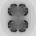
修改後的分解
整個動力平面的修改後的二進位制分解，圓形 Julia 集。帶有原始碼的影像
二進位制分解的另一種修改
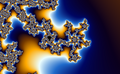
帶有樹枝狀 Julia 集的動力平面的修改後的分解。帶有原始碼的影像
帶有巴西利卡 Julia 集的動力平面的修改後的分解。帶有原始碼的影像

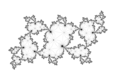
這裡 Julia 集的外部被分解成徑向水平集。

這是因為主迴圈沒有跳出測試，並且迭代次數（迭代最大值）是恆定的。

它建立了徑向水平集。

另請參閱

mandel：演算法 9 = qn(c) 的零點
bryceguy72 的影片^[15]
FreymanArt 的影片^[16]

  for (Iteration=0;Iteration<8;Iteration++)
 /* modified loop without checking of abs(zn) and low iteration max */
    {
    Zy=2*Zx*Zy + Cy;
    Zx=Zx2-Zy2 +Cx;
    Zx2=Zx*Zx;
    Zy2=Zy*Zy;
   };
  iTemp=((iYmax-iY-1)*iXmax+iX)*3;        
  /* --------------- compute  pixel color (24 bit = 3 bajts) */
 /* exterior of Filled-in Julia set  */
 /* binary decomposition  */
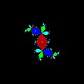
  if (Zy>0 ) 
   { 
    array[iTemp]=255; /* Red*/
    array[iTemp+1]=255;  /* Green */ 
    array[iTemp+2]=255;/* Blue */
  }
  if (Zy<0 )
   {
    array[iTemp]=0; /* Red*/
    array[iTemp+1]=0;  /* Green */ 
    array[iTemp+2]=0;/* Blue */    
  };

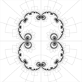
它也與莫比烏斯變換群的自同構函式有關 ^[17]

吸引域中的 BDM

吸引域中的 BDM（通常是 Julia 集的內部）給出了（偽）場線

解釋由 Gert Buschmann

形式為 ${\frac {(1-z^{3}/6)}{(z-z^{2}/2)^{2}}}+c$ 的迭代的場線。

在每個 Fatou 域（不是中性的）中，有兩個相互垂直的線系：等勢線（用於勢函式或實數迭代次數）和場線。

如果我們根據迭代次數（而不是實數迭代次數 $\nu (z)$ ，如上一節所定義）對 Fatou 域進行著色，則迭代的帶顯示了等勢線的路徑。如果迭代趨於 ∞（就像通常迭代 $z^{2}+c$ 的外部 Fatou 域中那樣），我們可以很容易地顯示場線的路徑，即根據迭代序列中的最後一個點在x軸上方還是下方來改變顏色（第一張圖片），但在這種情況下（更確切地說：當 Fatou 域是超吸引時），我們無法連貫地繪製場線 - 至少不能透過我們在這裡描述的方法。在這種情況下，場線也稱為外部射線。

設z為吸引 Fatou 域中的一個點。如果我們對z進行大量的迭代，迭代序列的終點是一個有限迴圈C，而 Fatou 域（根據定義）是迭代序列收斂於C的點的集合。場線從C的點以及迭代到C中的點的（無限多個）點發出。它們在 Julia 集中結束於非混沌點（即生成有限迴圈的點）。設r為迴圈C的階數（其點的數量），設z*為C中的一個點。我們有 $f(f(\dots f(z^{*})))=z^{*}$ （r 次複合），我們定義複數 α 為

\alpha =(d(f(f(\dots f(z))))/dz)_{z=z^{*}}.

如果C的點是 $z_{i},i=1,\dots ,r(z_{1}=z^{*})$ ，α 是r 個數 $f'(z_{i})$ 的乘積。實數 1/|α| 是迴圈的吸引力，我們假設迴圈既不中性也不超吸引，這意味著 1 < 1/|α| < ∞。點z* 是 $f(f(\dots f(z)))$ 的不動點，在這個點附近，對映 $f(f(\dots f(z)))$ 具有（與場線相關的）旋轉的特徵，旋轉的角度為 α 的幅角 β（即 $\alpha =|\alpha |e^{\beta i}$ ）。

為了給 Fatou 域著色，我們選擇了一個小的數字 ε，並設定迭代序列 $z_{k}(k=0,1,2,\dots ,z_{0}=z)$ 在 $|z_{k}-z^{*}|<\epsilon$ 時停止，我們根據數字k（或者如果我們希望平滑著色，則根據實際迭代次數）對點z 著色。如果我們從z* 選擇一個由角度 θ 給出的方向，則從z* 以這個方向發出的場線由以下點z 組成：數 $z_{k}-z^{*}$ 的幅角 ψ 滿足以下條件：

\psi -k\beta =\theta \mod \pi .\,

如果我們在場線方向（遠離迴圈）上透過一個迭代帶，則迭代次數k增加 1，而數字 ψ 增加 β，因此數字 $\psi -k\beta \mod \pi$ 沿場線保持恆定。

對 Fatou 域場線的著色意味著我們對場線對之間的空間進行著色：我們選擇從 z* 發出的幾個規則分佈的方向，並在每個方向上選擇兩個圍繞該方向的方向。由於場線對的兩個場線可能不會在 Julia 集的同一點結束，因此我們著色的場線在它們通往 Julia 集的路上可以（無限地）分叉。我們可以根據到場線中心線的距離進行著色，並且可以將這種著色與通常的著色混合在一起。這種圖片可以非常裝飾性（第二張圖片）。

一條著色的場線（兩條場線之間的區域）被迭代帶劃分，這樣一部分可以與單位正方形建立一一對應關係：一個座標是（從）到其中一條邊界場線的距離計算出來的，另一個座標是（從）到邊界迭代帶的內側距離計算出來的（這個數字是實迭代次數的非整數部分）。因此，我們可以將圖片放入場線中（第三張圖片）。

待辦事項

將斜率新增到白色

逆迭代法 (IIM/J) : Julia 集

斥點的逆迭代用於繪製 Julia 集

復勢 - Boettcher 座標

此處檢視描述

DEM/J

該演算法有兩個版本

將它與引數平面和 Mandelbrot 集的版本 : DEM/M 進行比較。它與 M 集外部距離估計相同，但使用對 Z 的導數而不是對 C 的導數。

收斂

在這個演算法中，檢查同一個軌道上兩個點的距離

軌道的平均離散速度

它在以下情況下使用

柯西收斂演算法 (CCA)

該演算法由使用者：Georg-Johann 描述。這裡還有 Paul Nylander 編寫的 Matemathics 程式碼

正規性

正規性在此演算法中，檢查兩個軌道上點的距離

Michael Becker 檢查等連續性

"迭代在 Fatou 集上是等連續的，而在 Julia 集上則不是"。（Wolf Jung）^[18]^[19]

Michael Becker 在黎曼球面上比較了迭代下兩個靠近點的距離。^[20]^[21]

此方法不僅可以用於繪製多項式的 Julia 集（其中無窮大始終是超吸引不動點），還可以應用於其他函式（對映），其中無窮大不是吸引不動點。^[22]

使用 Wolf Jung 的 Marty 準則

Wolf Jung 正在使用“一種檢查正規性的替代方法，它基於 Marty 的準則：|f'| / (1 + |f|^2) 對於所有迭代必須有界”。它在 mndlbrot::marty 函式中實現（請參閱程式 Mandel 版本 5.3 的原始碼）。它使用動態平面上的一點。

科尼格斯座標

科尼格斯座標用於有限吸引（非超吸引）點（迴圈）的吸引盆中。

最佳化

距離

你不需要平方根來比較距離。^[23]

對稱

Julia 集可以具有許多對稱性 ^[24]^[25]

二次 Julia 集始終具有旋轉對稱性（180 度）

colour(x,y) = colour(-x,-y)

當 c 位於實軸上（cy = 0）時，Julia 集也具有反射對稱性：^[26]

colour(x,y) = colour(x,-y)

演算法

計算一半影像
旋轉並新增另一半
將影像寫入檔案 ^[27]

顏色

計算機圖形中的顏色
- 顏色理論/顏色漸變
Georg-Johann 對 Julia 集的視覺化
Chris King 對 Julia 集和引數平面的聯合描繪方法
關於分形著色技術 Jussi Harkonen 碩士論文，Åbo Akademi 大學數學系，圖爾庫，2007 年，61 頁。論文是在教授 Goran Hognas 的指導下完成的
技術資訊 - 由 Michael Condron 著色
Shawn Hargreaves 的 Technicolor Julias

集

目標集

前向軌道的陷阱
它是一個集合，可以捕獲任何趨於固定點/ 週期點的軌道。

Julia 集

"大多數用於計算 Julia 集的程式在基礎動力學是雙曲的時執行良好，但在拋物線情況下會遇到指數級減速。"（Mark Braverman）^[28]

當 Julia 集是不會在二次對映迭代下逃逸到無窮大的點集時（= 填充的 Julia 集沒有內部 = dendrt）
- IIM/J
- DEM/J
- 檢查正態性
當 Julia 集是兩個吸引盆之間的邊界時（= 填充的 Julia 集沒有空的內部）
- 邊界掃描 ^[29]
- 邊緣檢測

Fatou 集

填充的 Julia 集的內部可以被著色

吸引速度（整數值 = 用於猜測點是否在集合中的迭代次數），它被轉換為顏色（或灰色陰影） ^[30]
- 內部水平集
- 吸引時間（類似於逃逸時間，但檢查是否（abs(z-attractor)<Attracting_radius
- 二進位制分解
- Tomoki KAWAHIRA 對填充的 Julia 集內部的鑲嵌 ^[31]
Siegel 盤情況下的離散速度

週期點

更多內容請檢視這裡

影片

可以使用製作影片

放大動態平面
沿引數平面內的路徑更改引數 c ^[32]
更改著色方案（例如顏色迴圈）

示例

參考文獻

↑ Mark Braverman 和 Michael Yampolsky 的 Julia 集的可計算性
↑ 來自 Ultra Fractal 的標準著色演算法
↑ 新分形論壇 : 曼德爾布羅集的最低最佳逃逸值/
↑ math.stackexchange 問題：多項式的逃逸半徑及其填充的 Julia 集
↑ Bruce Dawson（Fractal eXtreme 的作者）的透過代數實現更快的分形
↑ 來自 tensorpudding 的使用 gsl 的 C 程式碼
↑ Wolf Jung 在 GNU 通用公共許可證下的程式 Mandel
↑ R. Grothmann 的 Euler 示例
↑ 透過逃逸線方法繪製曼德爾布羅集。M. Romera 等人
↑ Julia 曲線，曼德爾布羅集，Harold V. McIntosh。
↑ PythonDataScienceHandbook：Jake VanderPlas 的密度和等高線圖
↑ math.stackexchange 問題：等高線表示什麼
↑ Rodolphe Vaillant 的等高線
↑ E Demidov 的不動點和週期軌道
↑ 影片 : bryceguy72 的 Julia 集與磁場線的變形
↑ 影片 : FreymanArt 的用色帶/條紋變形 Julia 集
↑ Gerard Westendorp : 黎曼曲面的柏拉圖式鑲嵌 - 8 次迭代自同態函式 z->z^2 -0.1+ 0.75i
↑ Alan F. Beardon, S. Axler, F.W. Gehring, K.A. Ribet : 有理函式迭代：複分析動力系統。Springer，2000 年；ISBN 0387951512，9780387951515；第 49 頁
↑ Joseph H. Silverman : 動力系統的算術。Springer，2007 年。 ISBN 0387699031，9780387699035；第 22 頁
↑ Georg-Johann 視覺化 Julia 集
↑ 問題 : 在迭代下，兩個相近點的距離如何變化？如果我知道這一點，我能判斷這些點屬於哪個集合嗎？
↑ Michael Becker 的 Julia 集。請檢視度量 d(z,w)
↑ 演算法 : wikibooks 中的距離近似
↑ Evgeny Demidov 的 Julia 集對稱性
↑ mathoverflow : z2c 的 Julia 集對稱性
↑ htJulia Jewels：Michael McGoodwin 對 Julia 集的探索 (2000 年 3 月)
↑ Jonas Lundgren 在 Matlab 中的 Julia 集
↑ Mark Braverman : 關於拋物線 Julia 集的有效計算
↑ 拋物線不動點情況下的 Julia 集計算機建模演算法 N.B.Ampilova，E.Petrenko
↑ Keenan Crane 在 GPU 上的射線追蹤四元數 Julia 集
↑ Tomoki Kawahira 對填充的 Julia 集內部的鑲嵌
↑ devianart 上的 Julia 集動畫

Drakopoulos V.，比較 Julia 集的渲染方法，WSCG 雜誌 10 (2002)，155–161
Nathaniel D. Emerson 的動力學樹
"Julia 集和相關集合中的螺旋結構"，M. Michelitsch 和 O. E. Roessler 在一本書中 : 螺旋對稱 I. Hargittai 和 C. Pickover。(1992) 世界科學出版社，
"Julia 集中三臂螺旋的演化，以及更高階螺旋"，A. G. Davis Philip 在一本書中 : 螺旋對稱 I. Hargittai 和 C. Pickover。(1992) 世界科學出版社，
Beardon，A. : Julia 集的對稱性。數學情報員。1996-03-01 Springer 紐約 ISSN: 0343-6993 第 43 - 44 頁。

[1] Mark Braverman 和 Michael Yampolsky 的 Julia 集的可計算性

[2] 來自 Ultra Fractal 的標準著色演算法

[3] 新分形論壇 : 曼德爾布羅集的最低最佳逃逸值/

[4] th.stackexchange 問題：多項式的逃逸半徑及其填充的 Julia 集

[5] Bruce Dawson（Fractal eXtreme 的作者）的透過代數實現更快的分形

[6] 來自 tensorpudding 的使用 gsl 的 C 程式碼

[7] Wolf Jung 在 GNU 通用公共許可證下的程式 Mandel

[8] R. Grothmann 的 Euler 示例

[9] 透過逃逸線方法繪製曼德爾布羅集。M. Romera 等人

[10] Julia 曲線，曼德爾布羅集，Harold V. McIntosh。

[11] PythonDataScienceHandbook：Jake VanderPlas 的密度和等高線圖

[12] th.stackexchange 問題：等高線表示什麼

[13] Rodolphe Vaillant 的等高線

[14] E Demidov 的不動點和週期軌道

[15] 影片 : bryceguy72 的 Julia 集與磁場線的變形

[16] 影片 : FreymanArt 的用色帶/條紋變形 Julia 集

[17] Gerard Westendorp : 黎曼曲面的柏拉圖式鑲嵌 - 8 次迭代自同態函式 z->z^2 -0.1+ 0.75i

[18] Alan F. Beardon, S. Axler, F.W. Gehring, K.A. Ribet : 有理函式迭代：複分析動力系統。Springer，2000 年；ISBN 0387951512，9780387951515；第 49 頁

[19] Joseph H. Silverman : 動力系統的算術。Springer，2007 年。 ISBN 0387699031，9780387699035；第 22 頁

[20] Georg-Johann 視覺化 Julia 集

[21] 問題 : 在迭代下，兩個相近點的距離如何變化？如果我知道這一點，我能判斷這些點屬於哪個集合嗎？

[22] Michael Becker 的 Julia 集。請檢視度量 d(z,w)

[23] 演算法 : wikibooks 中的距離近似

[24] Evgeny Demidov 的 Julia 集對稱性

[25] thoverflow : z2c 的 Julia 集對稱性

[26] tJulia Jewels：Michael McGoodwin 對 Julia 集的探索 (2000 年 3 月)

[27] Jonas Lundgren 在 Matlab 中的 Julia 集

[28] Mark Braverman : 關於拋物線 Julia 集的有效計算

[29] 拋物線不動點情況下的 Julia 集計算機建模演算法 N.B.Ampilova，E.Petrenko

[30] Keenan Crane 在 GPU 上的射線追蹤四元數 Julia 集

[31] Tomoki Kawahira 對填充的 Julia 集內部的鑲嵌

[32] vianart 上的 Julia 集動畫

[1]

[2]

[3]

[4]

[5]

[6]

[7]

[8]

[9]

[10]

[11]

[12]

[13]

[14]

[15]

[16]

[17]

[18]

[19]

[20]

[21]

[22]

[23]

[24]

[25]

[26]

[27]

[28]

[29]

[30]

[31]

[32]

演算法