
分形/複平面迭代/拋物線
"大多數用於計算 Julia 集的程式在底層動力學為雙曲線時工作良好,但在拋物線情況下會遇到指數級減速。" (Mark Braverman)[1]
換句話說,這意味著使用標準/樸素演算法可能需要幾天時間才能製作出拋物線 Julia 集的優質影像。
這裡有兩個問題
- 緩慢(= 懶惰)的區域性動力學(在拋物線不動點附近)
- 某些部分非常薄(使用標準平面掃描很難找到)


動態平面 = 復 z 平面

- Julia 集 是一個公共邊界:
- Fatou 集


另請參閱
- 填充的Julia集[3]

- 拋物線棋盤或棋盤
- 拋物線內爆
- Fatou 座標
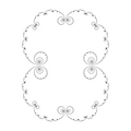
- 夏威夷耳環
- 維基百科中 = “由一系列圓形組成,所有圓形在同一處相切,且半徑序列收斂為零。”(MathWorld 的 Margherita Barile)[4]
- commons:Category:Hawaiian earrings
- Gevrey 漸近展開
- (7.1) 在原點的 Écalle-Voronin 不變數具有 Gevrey- 1/2 漸近展開[5]
- 胚芽[6][7][8]
- 函式的胚芽:函式的泰勒展開
- 重數[9]
- Julia-Lavaurs 集
- Leau-Fatou 花定理:[10] 排斥或吸引花。花由花瓣組成
- Leau-Fatou 花
- 拋物線線性化定理
- 喇叭對映
- Blaschke 積
- Inou 和 Shishikura 的近拋物線重整化
- 復多項式向量場[11]
- 數字
- “一個正整數 ν,即 **拋物線退化**,具有以下性質:存在 νq 個吸引花瓣和 νq 個排斥花瓣,它們圍繞不動點交替迴圈。”[12]
- 組合旋轉數
- 函式 f 在拋物線不動點處的龐加萊線性化器[13]
- “拋物線鉛筆。這是一個圓族,它們都有一個共同點,因此彼此相切,內部或外部。”[14]
Leau-Fatou 花定理指出,如果函式 具有泰勒展開[15]


則複數 在單位圓上 描述單位向量(方向)


- 如果 ,則 f 在原點處的排斥向量(從原點到 v)
- 如果 ,則吸引向量(從 v 到原點)


存在 n 個等距的吸引方向,由 n 個等距的排斥方向隔開。整數 n+1 稱為不動點的重數
%3Dz%5E2_%2B_mz_where_p_over_q%3D1_over_3.svg)
函式展開:z+z^5
/* Maxima CAS */
display2d:false;
taylor(z+z^5, z,0,5);

z + z^5
所以
- a = 1
- n = 4
計算吸引方向
/* Maxima CAS */
solve (4*v^4 = 1, v);

[v = %i/sqrt(2),v = -1/sqrt(2),v = -%i/sqrt(2),v = 1/sqrt(2)]
函式 m*z+z^2
(%i7) taylor(m*z+z^2, z,0,5);
(%o7) m*z+z^2
所以
- a = 1
- n = 1
(%i9) solve (v = 1, v);
(%o9) [v = 1]
Ecalle 柱面[16] 或 Ecalle-Voronin 柱面(由 Jean Ecalle[17][18])[19]
“... 在將 z 和 f(z) 等同(如果 z 和 f(z) 都屬於 P)的等價關係下,花瓣 P 的商。這個商流形稱為 Ecalle 柱面,它與無限柱面 C/Z 構形同構。”[20]
-
 手動打蛋器
手動打蛋器 -
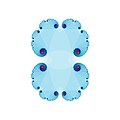
 以下是對拋物線情況下發生的真實模型


物理模型:使用打蛋器時蛋糕的行為。
數學模型:具有 2 箇中心(二階退化點)的二維向量場[21][22]
該場圍繞中心旋轉,但似乎沒有發散。
也許對拋物線動力學的更好描述是夏威夷耳環
- z+z^2
- z+z^3
- z+z^{k+1}
- z+a_{k+1}z^{k+1}
- z+a_{k+1}z^{k+1}
- "胚芽 與
≠ 0 , 1 {\displaystyle \vert a_{1}\vert \neq 0,1} 透過全純共軛到其線性部分 " (Sylvain Bonnot)[26]

 透過全純共軛到其線性部分
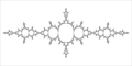
向量場的胚芽
"喇叭對映 h = Φ ◦ Ψ,其中 Φ 是 Φattr 的簡寫,Ψ 是 Ψrep 的簡寫(擴充套件的 Fatou 座標和引數化)。"[27]

_%3D_z%2Ba_2z_%5E2%2BO(z%5E3).png)

定義
- 萼片是吸引花瓣和排斥花瓣的交點。拋物線 Pommerenke-Levin-Yoccoz 不等式。由 Xavier Buf 和 Adam L. Epstein 似乎沒有萼片的正式定義。
- "設 l 是第一象限中的不變曲線,L1 是 l ∪ {0} 包圍的區域,稱為萼片。"[29]
- 包含拋物線不動點的邊界上的分量的內部
-
 Lea-Fatu 花
 -
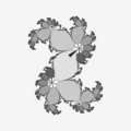
 具有四個花瓣和中心為拋物線點的花
 -
 內部角為 1/5 的臨界軌道,顯示 5 個吸引方向


所有 花瓣 的總和形成一朵花[30],中心位於拋物線週期點。[31]
花椰菜或西蘭花:[32]
- 空(其內部為空)對於 Mandelbrot 集之外的 c。Julia 集是完全不連通的。
- 對於 Mandelbrot 集邊界上的 c=1/4,填充的花椰菜。Julia 集是 Jordan 曲線(準圓)。
-
 c = 0 < 1/4
 -
 c = 0.25 = 1/4 是主心形的根。Julia 集是花椰菜。
 -
 c = 0.255 > 1/4 "內爆的花椰菜"
 -
 c = 0.258 > 1/4
 -
![c = [0.285, 0.01]](//upload.wikimedia.org/wikipedia/commons/thumb/1/17/Julia_set_%28highres_01%29.jpg/120px-Julia_set_%28highres_01%29.jpg) c = [0.285, 0.01]
c = [0.285, 0.01]


.jpg)
![c = [0.285, 0.01]](/wiki/File:Julia_set_(highres_01).jpg)
請注意
- 影像大小因 z 平面不同而異。
- 使用了不同的演算法,因此顏色很難比較。
Julia 集如何沿著實軸變化(從 c=0 到 c=1/4,然後更遠)
擾動函式 由複數


當新增一個大於0的ε(沿實軸向正無窮大移動)時,會出現一個拋物型不動點的分叉
- 吸引不動點 (ε<0)
- 一個拋物型不動點 (ε = 0)
- 一個拋物型不動點分裂成兩個共軛排斥不動點 (ε > 0)
“如果我們用ε<0稍微擾動,那麼拋物型不動點將在實軸上分裂成兩個實不動點(一個吸引,一個排斥)。”
參見
- Wolf Jung 的 Mandel 程式中的演示 2,第 9 頁
拋物線內爆
[edit | edit source]拋物型內爆
- 在引數平面中
- 點 c 從分量的內部,穿過邊界,到曼德爾布羅特集的外部
- 核 (c=0),沿內部射線 0,拋物點 (c= 0.25),沿外部射線 0
- 在動力學平面中
- 連線的朱利亞集(有內部)內爆,並斷開連線(沒有內部)
- 不動點從內部移動到朱利亞集(拋物型)
- 一個盆地(內部)消失
| 引數 c | 位置 | 朱利亞集 | 內部 | 動力學型別 | 臨界點 | 不動點 |
|---|---|---|---|---|---|---|
| c = 0 | 中心,內部 | 連線的 | 存在 | 超吸引 | 被吸引到 alfa 不動點 | 固定臨界點等於 alfa 不動點,alfa 是超吸引的,beta 是排斥的 |
| 0<c<1/4 | 內部射線 0,內部 | 連線的 | 存在 | 吸引 | 被吸引到 alfa 不動點 | alfa 是吸引的,beta 是排斥的 |
| c = 1/4 | 尖點,邊界 | 連線的 | 存在 | 拋物型 | 被吸引到 alfa 不動點 | alfa 不動點等於 beta 不動點,兩者都是拋物型的 |
| c>1/4 | 外部射線 0,外部 | 斷開連線的 | 消失 | - | 排斥到無窮大 | 兩個有限不動點都是排斥的 |
%3Dz*z_%2Bc.gif)

YouTube 上的影片[33]
- 拋物型內爆:從圓形到花椰菜,再到內爆的花椰菜
-
c=0
-
c=1/4
-
c= 1/4 + 0.05
-
 c = 1/4 + 0.029
 -
c = 1/4 + 0.035

向量場
[edit | edit source]- 二維向量場及其
奇點
[edit | edit source]奇點型別
“曲線扇區定義為由半徑任意小的圓 C 和兩個流線 S 和 S! 圍成的區域,這兩個流線都收斂到奇點。然後考慮透過開扇區 g 的流線,以區分三種可能的曲線扇區型別。”
動力學
[edit | edit source]動力學
- 全域性
- 區域性
區域性動力學
- 在朱利亞集的外部
- 在朱利亞集上
- 靠近拋物型不動點(在朱利亞集內部)
另請參閱
靠近拋物型不動點
[edit | edit source]
為什麼分析 f^p 而不是 f?
f 靠近拋物型不動點的正向軌道是複合的。它由兩種運動組成
- 圍繞不動點
- 向不動點移動/遠離不動點
如何計算拋物型 c 值
[edit | edit source]拋物型引數的型別
- 根點
- 尖點
| n | 內部角(旋轉數)t = 1/n | 根點 c = 拋物型引數 | 落在根點 c 上的引數射線的兩個外部角(1/(2^n+1); 2/(2^n+1) | 不動點 | 落在不動點 |
|---|---|---|---|---|---|
| 1 | 1/1 | 0.25 | (0/1 ; 1/1) | 0.5 | (0/1 = 1/1) |
| 2 | 1/2 | -0.75 | (1/3; 2/3) | -0.5 | (1/3; 2/3) |
| 3 | 1/3 | 0.64951905283833*%i-0.125 | (1/7; 2/7) | 0.43301270189222*%i-0.25 | (1/7; 2/7; 3/7) |
| 4 | 1/4 | 0.5*%i+0.25 | (1/15; 2/15) | 0.5*%i | (1/15; 2/15; 4/15; 8/15) |
| 5 | 1/5 | 0.32858194507446*%i+0.35676274578121 | (1/31; 2/31) | 0.47552825814758*%i+0.15450849718747 | (1/31; 2/31; 4/31; 8/31; 16/31) |
| 6 | 1/6 | 0.21650635094611*%i+0.375 | (1/63; 2/63) | 0.43301270189222*%i+0.25 | (1/63; 2/63; 4/63; 8/63; 16/63; 32/63) |
| 7 | 1/7 | 0.14718376318856*%i+0.36737513441845 | (1/127; 2/127) | 0.39091574123401*%i+0.31174490092937 | (1/127; 2/127, 4/127; 8/127; 16/127; 32/127, 64/127) |
| 8 | 1/8 | 0.10355339059327*%i+0.35355339059327 | 0.35355339059327*%i+0.35355339059327 | ||
| 9 | 1/9 | 0.075191866590218*%i+0.33961017714276 | 0.32139380484327*%i+0.38302222155949 | ||
| 10 | 1/10 | 0.056128497072448*%i+0.32725424859374 | 0.29389262614624*%i+0.40450849718747 |

對於內部角 n/p 拋物週期 p 迴圈,它包含一個具有 p 重數的 z 點[36] 和一個乘子 = 1.0。這個點 z 等於不動點

週期 1
[edit | edit source]可以輕鬆計算邊界點 c

對於給定的內部角(旋轉數)t,使用 Wolf Jung 編寫的這段cpp 程式碼[37]
 t *= (2*PI); // from turns to radians
 cx = 0.5*cos(t) - 0.25*cos(2*t);
 cy = 0.5*sin(t) - 0.25*sin(2*t);
或這段 Maxima CAS 程式碼
/* conformal map from circle to cardioid ( boundary
 of period 1 component of Mandelbrot set */
F(w):=w/2-w*w/4;

/*
circle D={w:abs(w)=1 } where w=l(t,r)
t is angle in turns ; 1 turn = 360 degree = 2*Pi radians
r is a radius
*/
ToCircle(t,r):=r*%e^(%i*t*2*%pi);

GiveC(angle,radius):=
(
 [w],
 /* point of  unit circle   w:l(internalAngle,internalRadius); */
 w:ToCircle(angle,radius),  /* point of circle */
 float(rectform(F(w)))    /* point on boundary of period 1 component of Mandelbrot set */
)$

compile(all)$

/* ---------- global constants & var ---------------------------*/
Numerator: 1;
DenominatorMax: 10;
InternalRadius: 1;

/* --------- main -------------- */
for Denominator:1 thru DenominatorMax step 1 do
(
 InternalAngle: Numerator/Denominator,
 c: GiveC(InternalAngle,InternalRadius),
 display(Denominator),
 display(c),
  /* compute fixed point */
 alfa:float(rectform((1-sqrt(1-4*c))/2)), /* alfa fixed point */
 display(alfa)
)$
週期 2
[edit | edit source]// cpp code by W Jung http://www.mndynamics.com
t *= (2*PI); // from turns to radians
cx = 0.25*cos(t) - 1.0;
cy = 0.25*sin(t);
週期 1-6
[edit | edit source]/*
batch file for Maxima CAS
computing bifurcation points for period 1-6
Formulae for cycles in the Mandelbrot set II
Stephenson, John; Ridgway, Douglas T.
Physica A, Volume 190, Issue 1-2, p. 104-116.
*/
kill(all);
remvalue(all);
start:elapsed_run_time ();
/* ------------ functions ----------------------*/
/* exponential for of complex number with angle in turns */
/* "exponential form prevents allroots from working", code by Robert P. Munafo */
GivePoint(Radius,t):=rectform(ev(Radius*%e^(%i*t*2*%pi), numer))$ /* gives point of unit circle for angle t in turns */
GiveCirclePoint(t):=rectform(ev(%e^(%i*t*2*%pi), numer))$ /* gives point of unit circle for angle t in turns Radius = 1 */
/* gives a list of iMax points of unit circle */
GiveCirclePoints(iMax):=block(
[circle_angles,CirclePoints],
CirclePoints:[],
circle_angles:makelist(i/iMax,i,0,iMax),
for t in circle_angles do CirclePoints:cons(GivePoint(1,t),CirclePoints),
return(CirclePoints) /* multipliers */
)$
/* http://commons.wikimedia.org/wiki/File:Mandelbrot_set_Components.jpg
Boundary equation b_n(c,P)=0
defines relations between hyperbolic components and unit circle for given period n ,
allows computation of exact coordinates of hyperbolic componenets.
b_n(w,c), is boundary polynomial (implicit function of 2 variables).
*/
GiveBoundaryEq(P,n):=
block(
if n=1 then return(c + P^2 - P),
if n=2 then return(- c + P - 1),
if n=3 then return(c^3 + 2*c^2 - (P-1)*c + (P-1)^2),
if n=4 then return(c^6 + 3*c^5 + (P+3)* c^4 + (P+3)* c^3 - (P+2)*(P-1)*c^2 - (P-1)^3),
if n=5 then return(c^15 + 8*c^14 + 28*c^13 + (P + 60)*c^12 + (7*P + 94)*c^11 +
(3*P^2 + 20*P + 116)*c^10 + (11*P^2 + 33*P + 114)*c^9 + (6*P^2 + 40*P + 94)*c^8 +
(2*P^3 - 20*P^2 + 37*P + 69)*c^7 + (3*P - 11)*(3*P^2 - 3*P - 4)*c^6 + (P - 1)*(3*P^3 + 20*P^2 - 33*P - 26)*c^5 +
(3*P^2 + 27*P + 14)*(P - 1)^2*c^4 - (6*P + 5)*(P - 1)^3*c^3 + (P + 2)*(P - 1)^4*c^2 - c*(P - 1)^5 + (P - 1)^6),
if n=6 then return (c^27+
13*c^26+
78*c^25+
(293 - P)*c^24+
(792 - 10*P)*c^23+
(1672 - 41*P)*c^22+
(2892 - 84*P - 4*P^2)*c^21+
(4219 - 60*P - 30*P^2)*c^20+
(5313 + 155*P - 80*P^2)*c^19+
(5892 + 642*P - 57*P^2 + 4*P^3)*c^18+
(5843 + 1347*P + 195*P^2 + 22*P^3)*c^17+
(5258 + 2036*P + 734*P^2 + 22*P^3)*c^16+
(4346 + 2455*P + 1441*P^2 - 112*P^3 + 6*P^4)*c^15 +
(3310 + 2522*P + 1941*P^2 - 441*P^3 + 20*P^4)*c^14 +
(2331 + 2272*P + 1881*P^2 - 853*P^3 - 15*P^4)*c^13 +
(1525 + 1842*P + 1344*P^2 - 1157*P^3 - 124*P^4 - 6*P^5)*c^12 +
(927 + 1385*P + 570*P^2 - 1143*P^3 - 189*P^4 - 14*P^5)*c^11 +
(536 + 923*P - 126*P^2 - 774*P^3 - 186*P^4 + 11*P^5)*c^10 +
(298 + 834*P + 367*P^2 + 45*P^3 - 4*P^4 + 4*P^5)*(1-P)*c^9 +
(155 + 445*P - 148*P^2 - 109*P^3 + 103*P^4 + 2*P^5)*(1-P)*c^8 +
2*(38 + 142*P - 37*P^2 - 62*P^3 + 17*P^4)*(1-P)^2*c^7 +
(35 + 166*P + 18*P^2 - 75*P^3 - 4*P^4)*((1-P)^3)*c^6 +
(17 + 94*P + 62*P^2 + 2*P^3)*((1-P)^4)*c^5 +
(7 + 34*P + 8*P^2)*((1-P)^5)*c^4 +
(3 + 10*P + P^2)*((1-P)^6)*c^3 +
(1 + P)*((1-P)^7)*c^2 +
-c*((1-P)^8) + (1-P)^9)
)$
/* gives a list of points c on boundaries on all components for give period */
GiveBoundaryPoints(period,Circle_Points):=block(
[Boundary,P,eq,roots],
Boundary:[],
for m in Circle_Points do (/* map from reference plane to parameter plane */
P:m/2^period,
eq:GiveBoundaryEq(P,period), /* Boundary equation b_n(c,P)=0 */
roots:bfallroots(%i*eq),
roots:map(rhs,roots),
for root in roots do Boundary:cons(root,Boundary)),
return(Boundary)
)$
/* divide llist of roots to 3 sublists = 3 components */
/* ---- boundaries of period 3 components
period:3$
Boundary3Left:[]$
Boundary3Up:[]$
Boundary3Down:[]$
Radius:1;
for m in CirclePoints do (
P:m/2^period,
eq:GiveBoundaryEq(P,period),
roots:bfallroots(%i*eq),
roots:map(rhs,roots),
for root in roots do
(
if realpart(root)<-1 then Boundary3Left:cons(root,Boundary3Left),
if (realpart(root)>-1 and imagpart(root)>0.5)
then Boundary3Up:cons(root,Boundary3Up),
if (realpart(root)>-1 and imagpart(root)<0.5)
then Boundary3Down:cons(root,Boundary3Down)
)
)$
--------- */
/* gives a list of parabolic points for given: period and internal angle */
GiveParabolicPoints(period,t):=block
(
[m,ParabolicPoints,P,eq,roots],
m: GiveCirclePoint(t), /* root of unit circle, Radius=1, angle t=0 */
ParabolicPoints:[],
/* map from reference plane to parameter plane */
P:m/2^period,
eq:GiveBoundaryEq(P,period), /* Boundary equation b_n(c,P)=0 */
roots:bfallroots(%i*eq),
roots:map(rhs,roots),
for root in roots do ParabolicPoints:cons(float(root),ParabolicPoints),
return(ParabolicPoints)
)$
compile(all)$
/* ------------- constant values ----------------------*/
fpprec:16;
/* ------------unit circle on a w-plane -----------------------------------------*/
a:GiveParabolicPoints(6,1/3);
a$
/*
gcc c.c -lm -Wall
./a.out
Root point between period 1 component and period 987 component  = c = 0.2500101310666710+0.0000000644946597
Internal angle (c) = 1/987
Internal radius (c) = 1.0000000000000000

*/

#include <stdio.h>
#include <math.h>		// M_PI; needs -lm also
#include <complex.h>


/*
   c functions using complex type numbers
   computes c from  component  of Mandelbrot set */
complex double Give_c( int Period,  int n, int d , double InternalRadius )
{
  complex double c;
  complex double w;  // point of reference plane  where image of the component is a unit disk
 // alfa = ax +ay*i = (1-sqrt(d))/2 ; // result
  double t; // InternalAngleInTurns

  t  = (double) n/d;
  t = t * M_PI * 2.0; // from turns to radians

  w = InternalRadius*cexp(I*t); // map to the unit disk

  switch ( Period ) // of component
    {
    case 1: // main cardioid = only one period 1 component
      c = w/2 - w*w/4; // https://wikibook.tw/wiki/Fractals/Iterations_in_the_complex_plane/Mandelbrot_set/boundary#Solving_system_of_equation_for_period_1
      break;
    case 2: // only one period 2 component
      c = (w-4)/4 ; // https://wikibook.tw/wiki/Fractals/Iterations_in_the_complex_plane/Mandelbrot_set/boundary#Solving_system_of_equation_for_period_2
      break;
      // period > 2
    default:
      printf("higher periods : to do, use newton method \n");
      printf("for each q = Period of the Child component  there are 2^(q-1) roots \n");
      c = 10000.0; // bad value

      break; }


  return c;
}


void PrintAndDescribe_c( int period,  int n, int d , double InternalRadius ){


	complex double c = Give_c(period, n, d, InternalRadius);

	printf("Root point between period %d component and period %d component  = c = %.16f%+.16f*I\t",period, d, creal(c), cimag(c));
	printf("Internal angle (c) = %d/%d\n",n, d);
	//printf("Internal radius (c) = %.16f\n",InternalRadius);


}

/*
https://stackoverflow.com/questions/19738919/gcd-function-for-c
The GCD function uses Euclid's Algorithm.
It computes A mod B, then swaps A and B with an XOR swap.
*/

int gcd(int a, int b)
{
    int temp;
    while (b != 0)
    {
        temp = a % b;

        a = b;
        b = temp;
    }
    return a;
}


int main (){


	int period = 1;
	double InternalRadius = 1.0;
	// internal angle in turns as a ratio = p/q
	int n = 1;
	int d = 987;


	// n/d = local angle in turns

   		for (n = 1; n < d; ++n ){
     			if (gcd(n,d)==1 )// irreducible fraction
       				{ PrintAndDescribe_c(period, n,d,InternalRadius); }
       				}


	return 0;

}
- 5 種繪製方法
-
 檢查迭代次數
 -
 修改後的 DEM
 -
 檢查角度
檢查角度 -
 檢查 zn 是否在目標集內
 -
 檢查 zn 是否在三角形目標集內


填充朱利亞集內部的所有點都趨向於一個週期軌道(或不動點)。此點位於朱利亞集中,並且是弱吸引的。[38] 您可以分析拋物線不動點附近的行為。可以使用 臨界軌道 來完成此操作。
這裡有兩種情況:簡單和困難。
如果拋物線不動點附近的朱利亞集類似於 n 臂星形(未扭曲),則您可以簡單地檢查 zn 相對於不動點的幅角。例如,請參見 z+z^5。這是一個簡單的例子。
在困難的情況下,朱利亞集圍繞不動點扭曲。
根點的朱利亞集在拓撲上與子週期中心的朱利亞集相同,但
- 中心(核)朱利亞集非常容易繪製(超吸引盆 = 非常快的動態,因為臨界點也是週期點)
- 而根朱利亞集(拋物線)很難繪製(拋物線盆和懶惰動態)
示例
- t = 1/2
- 根點的朱利亞集 = 胖巴塞利卡朱利亞集:c = -3/4 = - 0.75
- 週期 2 中心的朱利亞集 = (細長)巴塞利卡朱利亞集:c = -1
- t = 1/3
描述
步驟
- 選擇函式 ,其在原點(z=0)處有一個固定拋物線點
- 選擇內部角度
- 計算 ,它是函式 的較高迭代次數的近似值,z 接近於零,使用以零為中心的冪級數(泰勒級數 = 麥克勞林級數)
- 實驗性地找出使用冪級數的項數以及使用特定 的環帶


每個 將被用於一個環帶

其中 K 為固定值
具有在原點處具有乘子 的無差異不動點的復二次多項式的 Lambda 形式[41]


其中
- 定點的乘數
- 內角是一個有理數和真分數

選擇
- 因此
- 冪級數的30項
- 環k=4,5,...,10的近似函式,對於z的較大值(在環外),使用預設函式f^n
- 函式的delta等於10^-5


(* code by Professor: Mark McClure from https://marksmath.org/classes/Spring2019ComplexDynamics/ *)
n = 7;
f[z_] = Exp[2 Pi*I/n] z + z^2;

Remove[F];
F[0][z_]    = N[Normal[Series[f[z], {z, 0, 30}]]];
Do[F[0][z_] = Chop[N[Normal[Series[F[0][f[z]], {z, 0, 30}]]], 10^-5],  {n - 1}];
Do[F[k][z_] = Chop[N[Normal[Series[F[k - 1][F[k - 1][z]], {z, 0, 30}]]], 10^-5], {k, 1, 10}]

(* define and compile function FF *)
FF = With[{
    n = n,
    f4 = Function[z, Evaluate[F[4][z]]],
    f5 = Function[z, Evaluate[F[5][z]]],
    f6 = Function[z, Evaluate[F[6][z]]],
    f7 = Function[z, Evaluate[F[7][z]]],
    f8 = Function[z, Evaluate[F[8][z]]],
    f9 = Function[z, Evaluate[F[9][z]]],
    f10 = Function[z, Evaluate[F[10][z]]]
    },
   Compile[{{z, _Complex}},
    Which[
     Abs[z] > 1/2^3,
     Nest[Function[zz, N[Exp[2 Pi*I/n]] zz + zz^2], z, n],
     Abs[z] <= 1/2^9, f10[z],
     Abs[z] <= 1/2^8, f9[z],
     Abs[z] <= 1/2^7, f8[z],
     Abs[z] <= 1/2^6, f7[z],
     Abs[z] <= 1/2^5, f6[z],
     Abs[z] <= 1/2^4, f5[z],
     Abs[z] <= 1/2^3, f4[z],
     True, 0]]];

(* iterate 1000 times and then see what happens *)
iterate = With[{FF = FF, n = n},
   Compile[{{z0, _Complex}},
    Module[{z, i},
     z = z0;
     i = 0;
     While[1/2^9 < Abs[z] <= 2 && i++ < 1000 n,
      z = FF[z]];
     z],
    RuntimeOptions -> "Speed", CompilationTarget -> "C"]];

(* now compute some iteration data *)
data = Monitor[
    Table[iterate[x + I*y], {y, Im[center] + 1.2, Im[center], -0.0025},
     {x, Re[center] - 1.2, Re[center] + 1.2, 0.0025}],
    y];


(* use some symmetry to cut computation time in half *)
center = First[Select[z /. NSolve[f[z] == 0, z], Im[#] < 0 &]]/2 (* center = -0.311745 - 0.390916*I *)
data = Join[data, Reverse[Rest[Reverse /@ data]]];


(* plot it  *)
kernel = {
   {1, 1, 1},
   {1, -8, 1},
   {1, 1, 1}
   };

 (*
classifyArg = Compile[
   {{z, _Complex}, {z0, _Complex}, {v, _Complex}, {n, _Integer}},
   Module[{check, check2},
    check = n (Arg[(z0 - z)/v] + Pi)/(2 Pi);
    check2 = Ceiling[check];
    If[check == check2, 0, check2]]];


classified = Map[classify, data, {2}];

convolvedData = ListConvolve[kernel, classified];

ArrayPlot[Sign[Abs[convolvedData]]]
Wolfram 語言的數學函式(
- Series[f,{x,x0,n}] 生成關於點的f的冪級數展開,階數為,其中n是一個明確的整數
- N[expr] 給出expr的數值
- Chop[expr,delta] 將絕對值小於delta的數字替換為0
- Normal[expr] 將expr從各種特殊形式轉換為正常表示式。
- Do[expr,n] 評估expr n次
- Do[expr,{i,imin,imax}] 評估expr,從i=imin開始
- With[{x=x0,y=y0,…},expr] 指定expr中所有x、y等的出現應該被替換為x0、y0等。
- Compile[{{x1,t1},…},expr] 假設xi的型別與ti匹配。
- Which[test1,value1,test2,value2,…] 依次評估每個testi,返回第一個產生True的valuei的值
- Nest[f,expr,n] 給出對expr應用n次f的表示式。


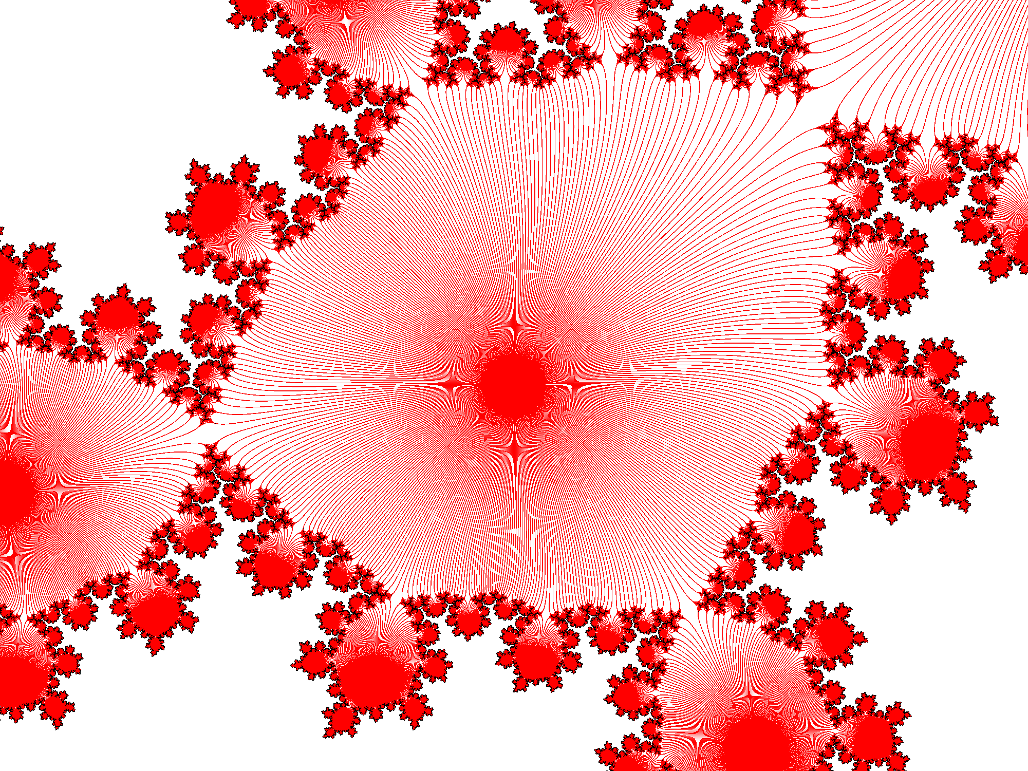
動態射線
[edit | edit source]
可以使用落在拋物線不動點的週期性動態射線來尋找外部的狹窄部分。
讓我們檢查外部半徑=4的週期性射線上的點需要多少次反向迭代才能到達距離拋物線不動點0.003的位置
| 週期 | 反向迭代 | 時間 |
|---|---|---|
| 1 | 340 | 0m0.021s |
| 2 | 55 573 | 0m5.517s |
| 3 | 8 084 815 | 13m13.800s |
| 4 | 1 059 839 105 | 1724m28.990s |
| C原始碼 - 點選右側檢視 |
|---|
| a.c |
/*
c console program
to compile:
 gcc double_t.c -lm -Wall -march=native

to run:
time ./a.out

period	EscapeTime	time
1	       340	 0m0.021s
2	    55 573   	 0m5.517s
3	 8 084 815	13m13.800s
4    1 059 839 105    1724m28.990s

period 1
escape time   = 340.000000
internal angle t  = 1.000000
period  = 1
preperiod  = 0
cx  = 0.250000
cy  = 0.000000
alfax  = 0.500000
alfay  = 0.000000
real	0m0.021s

===============
escape time   = 55573.000000
internal angle t  = 0.500000
period  = 2
preperiod  = 0
cx  = -0.750000
cy  = 0.000000
alfax  = -0.500000
alfay  = 0.000000

real	0m5.517s
===============================
period = 3  c = (-0.125000; 0.649519); alfa  = (-0.250000;0.433013)
ea  = 0.142857;
internal angle t  = 0.333333
preperiod  = 0
for period = 3  escape time =    8084815

real	13m13.800s
=====================================
period = 4  c = (0.250000; 0.500000); alfa  = (0.000000;0.500000)
ea  = 0.066667;
internal angle t  = 0.250000
preperiod  = 0
for period = 4  escape time = 1059839105

real	1724m28.990s

*/

#include <stdio.h>
#include <stdlib.h> // malloc
#include <math.h> // M_PI; needs -lm also
#include <complex.h>

unsigned int period = 4;// of child component of Mandelbrot set
unsigned int numerator=1 ;
unsigned int denominator;
double t ; // internal angle of point c of parent component of Mandelbrot set in turns
unsigned long int maxiter = 100000;
unsigned int preperiod = 0; //of external angle under doubling map

 double complex z , c, alfa;
  double ea ;// External Angle

/* find c in component of Mandelbrot set
 uses complex type so #include <complex.h> and -lm
 uses code by Wolf Jung from program Mandel
 see function mndlbrot::bifurcate from mandelbrot.cpp
 http://www.mndynamics.com/indexp.html

  */
double complex GiveC(double InternalAngleInTurns, double InternalRadius, unsigned int period)
{
  //0 <= InternalRay<= 1
  //0 <= InternalAngleInTurns <=1
  // period of parent component of Mandelbrot set  { 1,2 }
  double t = InternalAngleInTurns *2*M_PI; // from turns to radians
  double R2 = InternalRadius * InternalRadius;
  double Cx, Cy; /* C = Cx+Cy*i */
  switch ( period ) {
    case 1: // main cardioid
      Cx = (cos(t)*InternalRadius)/2-(cos(2*t)*R2)/4;
      Cy = (sin(t)*InternalRadius)/2-(sin(2*t)*R2)/4;
      break;
   case 2: // only one component
      Cx = InternalRadius * 0.25*cos(t) - 1.0;
      Cy = InternalRadius * 0.25*sin(t);
      break;
  // for each period  there are 2^(period-1) roots.
  default: // safe values
      Cx = 0.0;
      Cy = 0.0;
    break; }

  return Cx+ Cy*I;
}

/*

http://en.wikipedia.org/wiki/Periodic_points_of_complex_quadratic_mappings
z^2 + c = z
z^2 - z + c = 0
ax^2 +bx + c =0 // ge3neral for  of quadratic equation
so:
a=1
b =-1
c = c
so:

The discriminant is the d=b^2-4ac

d=1-4c = dx+dy*i
r(d)=sqrt(dx^2 + dy^2)
sqrt(d) = sqrt((r+dx)/2)+-sqrt((r-dx)/2)*i = sx +- sy*i

x1=(1+sqrt(d))/2 = beta = (1+sx+sy*i)/2

x2=(1-sqrt(d))/2 = alfa = (1-sx -sy*i)/2

alfa: attracting when c is in main cardioid of Mandelbrot set, then it is in interior of Filled-in Julia set, it means belongs to Fatou set (strictly to basin of attraction of finite fixed point)
*/
// uses global variables:
//  ax, ay (output = alfa(c))
double complex GiveAlfaFixedPoint(double complex c)
{
  double dx, dy; //The discriminant is the  d=b^2- 4ac = dx+dy*i
  double r; // r(d)=sqrt(dx^2 + dy^2)
  double sx, sy; // s = sqrt(d) = sqrt((r+dx)/2)+-sqrt((r-dx)/2)*i = sx + sy*i
  double ax, ay;

 // d=1-4c = dx+dy*i
 dx = 1 - 4*creal(c);
 dy = -4 * cimag(c);
 // r(d)=sqrt(dx^2 + dy^2)
 r = sqrt(dx*dx + dy*dy);
 //sqrt(d) = s =sx +sy*i
 sx = sqrt((r+dx)/2);
 sy = sqrt((r-dx)/2);
 // alfa = ax +ay*i = (1-sqrt(d))/2 = (1-sx + sy*i)/2
 ax = 0.5 - sx/2.0;
 ay =  sy/2.0;

return ax+ay*I;
}

double DistanceBetween(double complex z1, double complex z2)
{double dx,dy;

 dx = creal(z1) - creal(z2);
 dy = cimag(z1) - cimag(z2);
 return sqrt(dx*dx+dy*dy);

}

/*
 principal square  root of complex number
 http://en.wikipedia.org/wiki/Square_root

 z1= I;
  z2 = root(z1);
  printf("zx  = %f \n", creal(z2));
  printf("zy  = %f \n", cimag(z2));
*/
double complex root(double complex z)
{
  double x = creal(z);
  double y = cimag(z);
  double u;
  double v;
  double r = sqrt(x*x + y*y);

  v = sqrt(0.5*(r - x));
  if (y < 0) v = -v;
  u = sqrt(0.5*(r + x));
 return u + v*I;
}

double complex preimage(double complex z1, double complex z2,  double complex c)
{
  double complex zPrev;

  zPrev = root(creal(z1) - creal(c) + (cimag(z1) - cimag(c))*I);
  // choose one of 2 roots
  if (creal(zPrev)*creal(z2) + cimag(zPrev)*cimag(z2) > 0)
        return zPrev ;     //  u+v*i
       else return -zPrev; // -u-v*i
}

// This function only works for periodic or preperiodic angles.
// You must determine the period n and the preperiod k before calling this function.
// based on same function from src code of program Mandel by Wolf Jung
// http://www.mndynamics.com/indexp.html
double  backray(double t, // external angle in turns
		       int n, //period of ray's angle under doubling map
		       int k, // preperiod
                       int iterMax,
                       double complex c
                          )
{
  double xend ; // re of the endpoint of the ray
  double yend; // im of the endpoint of the ray
  const double R = 4; // very big radius = near infinity
  int j; // number of ray
  double iter=0.0; // index of backward iteration


  double complex zPrev;
  double u,v; // zPrev = u+v*I
  double complex zNext;
  double distance;

   /* dynamic 1D arrays for coordinates (x, y) of points with the same R on preperiodic and periodic rays  */
  double *RayXs, *RayYs;
  int iLength = n+k+2; // length of arrays ?? why +2
  //  creates arrays:  RayXs and RayYs  and checks if it was done
  RayXs = malloc( iLength * sizeof(double) );
  RayYs = malloc( iLength * sizeof(double) );
  if (RayXs == NULL || RayYs==NULL)
    {
      fprintf(stderr,"Could not allocate memory");
      getchar();
      return 1;
    }

 //  starting points on preperiodic and periodic rays
 //  with angles t, 2t, 4t...  and the same radius R
  for (j = 0; j < n + k; j++)
  { // z= R*exp(2*Pi*t)
    RayXs[j] = R*cos((2*M_PI)*t);
    RayYs[j] = R*sin((2*M_PI)*t);
    t *= 2; // t = 2*t
    if (t > 1) t--; // t = t modulo 1
  }
  zNext = RayXs[0] + RayYs[0] *I;

  //printf("RayXs[0]  = %f \n", RayXs[0]);
  //printf("RayYs[0]  = %f \n", RayYs[0]);

  // z[k] is n-periodic. So it can be defined here explicitly as well.
  RayXs[n+k] = RayXs[k];
  RayYs[n+k] = RayYs[k];

  //   backward iteration of each point z
  do
    {

        for (j = 0; j < n+k; j++) // period +preperiod
         { // u+v*i = sqrt(z-c)   backward iteration in fc plane
		zPrev = root(RayXs[j+1] - creal(c)+(RayYs[j+1] - cimag(c))*I); // , u, v
                u=creal(zPrev);
                v=cimag(zPrev);

		// choose one of 2 roots: u+v*i or -u-v*i
		if (u*RayXs[j] + v*RayYs[j] > 0)
                        { RayXs[j] = u; RayYs[j] = v; } // u+v*i
			else { RayXs[j] = -u; RayYs[j] = -v; } // -u-v*i
         } // for j ...

          //RayYs[n+k] cannot be constructed as a preimage of RayYs[n+k+1]
          RayXs[n+k] = RayXs[k];
          RayYs[n+k] = RayYs[k];

          // convert to pixel coordinates
          //  if z  is in window then draw a line from (I,K) to (u,v) = part of ray

       // printf("for iter = %d cabs(z) = %f \n", iter, cabs(RayXs[0] + RayYs[0]*I));
   iter += 1.0;
  distance = DistanceBetween(RayXs[j]+RayYs[j]*I, alfa);
   printf("distance  = %10.9f ; iter = %10.0f \n", distance, iter); // info
  }
 while (distance>0.003);// distance < pixel size

 // last point of a ray 0
 xend = RayXs[0];
 yend = RayYs[0];

 // free memmory
 free(RayXs);
 free(RayYs);

return  iter; //
}

/* ---------------------- main ------------------*/
int main()
{

 double EscapeTime;

  // internal angle
  denominator = period;
  t = (double) numerator/denominator;

  //
  c = GiveC(t, 1.0, 1);
  alfa = GiveAlfaFixedPoint(c);

  //external angle
  denominator= pow(2,period) - 1;
  ea = (double) 1.0/ denominator;
  //
  EscapeTime = backray(ea, period, preperiod, maxiter, c);


  //
  printf("period = %d ", period);
  printf(" c = (%f; %f);", creal(c), cimag(c));
  printf(" alfa  = (%f;%f)\n", creal(alfa), cimag(alfa));
  printf("ea  = %f;\n", ea);
  printf("internal angle t  = %f \n", t);
  printf("preperiod  = %d \n", preperiod);
  printf("for period = %d  escape time = %10.0f \n", period,  EscapeTime);
  //


  return 0;
}
|
可以使用外部射線的點z的幅角及其到alfa不動點的距離(參見影像中的程式碼)。它適用於週期數不超過15(也許更多……)。
從內部估計
[edit | edit source]朱利亞集是填充的朱利亞集Kc的邊界。
- 找到Kc內部的點
- 使用邊緣檢測找到Kc內部的邊界
如果內部的元件彼此非常接近,則使用以下方法找到元件:[42]
color = LastIteration % period
對於父元件和子元件之間的拋物線元件:[43]
periodOfChild = denominator*periodOfParent
color = iLastIteration % periodOfChild
其中分母是曼德勃羅集的父元件的內角的分母。
角度
[edit | edit source]"如果zn的迭代趨於一個固定的拋物點,那麼初始種子z0根據zn−z0的幅角進行分類,分類由花定理提供"(Mark McClure[44])
吸引時間
[edit | edit source]
填充的朱利亞集的內部由元件組成。所有元件都是前週期的,其中一些是週期的(吸引力的直接盆地)。
換句話說
- 一次迭代將z移動到另一個元件(以及整個元件移動到另一個元件)
- 所有元件的點都具有相同的吸引時間(到達吸引子周圍的目標集所需的迭代次數)
可以使用它來對元件進行著色。因為在拋物線情況下吸引子是弱的(弱吸引),所以某些點需要很多次迭代才能到達它。
 // i = number of iteration
 // iPeriodChild = period of child component of Mandelbrot set ( parabolic c value is a root point between parant and child component
 /* distance from z to Alpha  */
 Zxt=Zx-dAlfaX;
 Zyt=Zy-dAlfaY;
 d2=Zxt*Zxt +Zyt*Zyt;
 // interior: check if fall into internal target set (circle around alfa fixed point)
 if (d2<dMaxDistance2Alfa2) return  iColorsOfInterior[i % iPeriodChild];
這裡有一些示例值
 iWidth  = 1001 // width of image in pixels
 PixelWidth  = 0.003996
 AR  = 0.003996 // Radius around attractor
 denominator  = 1 ; Cx  = 0.250000000000000; Cy  = 0.000000000000000 ax  = 0.500000000000000; ay  = 0.000000000000000
 denominator  = 2 ; Cx  = -0.750000000000000; Cy  = 0.000000000000000 ax  = -0.500000000000000; ay  = 0.000000000000000
 denominator  = 3 ; Cx  = -0.125000000000000; Cy  = 0.649519052838329 ax  = -0.250000000000000; ay  = 0.433012701892219
 denominator  = 4 ; Cx  = 0.250000000000000; Cy  = 0.500000000000000 ax  = 0.000000000000000; ay  = 0.500000000000000
 denominator  = 5 ; Cx  = 0.356762745781211; Cy  = 0.328581945074458 ax  = 0.154508497187474; ay  = 0.475528258147577
 denominator  = 6 ; Cx  = 0.375000000000000; Cy  = 0.216506350946110 ax  = 0.250000000000000; ay  = 0.433012701892219

 denominator  = 1 ;   i =               243.000000
 denominator  = 2 ;   i =            31 171.000000
 denominator  = 3 ;   i =         3 400 099.000000
 denominator  = 4 ;   i =       333 293 206.000000
 denominator  = 5 ;   i =    29 519 565 177.000000
 denominator  = 6 ;   i = 2 384 557 783 634.000000
其中
C = Cx + Cy*i
a = ax + ay*i // fixed point alpha
i // number of iterations after which critical point z=0.0 reaches disc around fixed point alpha with radius AR
denominator of internal angle (in turns)
internal angle = 1/denominator
請注意,吸引時間i與分母成正比。

現在您看到了弱吸引意味著什麼。
你可以
- 使用蠻力方法(吸引半徑<畫素大小;迭代最大值足夠大,讓內部的所有點都到達目標集;長時間或快速計算機)
- 找到更好的方法(:-)),如果您覺得時間太長
內部距離估計
[edit | edit source]陷阱
[edit | edit source]
Julia 集是填充的 Julia 集和無窮大吸引域的共同邊界。
- 找到 Kc 內部/分量的點
- 找到逃逸點
- 使用 Sobel 濾波器找到邊界點
它適用於分母不超過 4。
逆迭代 阿爾法不動點。它只對切割點(外部射線落入的地方)有效。其他點仍然沒有被擊中。


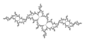
![1/2 San Marco fractal[45]](/wiki/File:Parabolic_julia_set_c%3D-0.75.png)
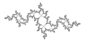
![1/3 Douady fat rabbit[46]](/wiki/File:Parabolic_Julia_set_for_internal_angle_1_over_3.png)


- 從週期 2 到 ...
-
![from 2 thru internal ray 1/1 ; c=-0.75 Julia set is a San Marco fractal[47]](//upload.wikimedia.org/wikipedia/commons/thumb/c/c5/Parabolic_julia_set_c%3D-0.75.png/120px-Parabolic_julia_set_c%3D-0.75.png) 從 2 到內部射線 1/1 ; c=-0.75 Julia 集是一個 聖馬可分形[47]
從 2 到內部射線 1/1 ; c=-0.75 Julia 集是一個 聖馬可分形[47] -
 從週期 2 到 1/2
 -
 從週期 2 到 1/3
 -
 從週期 2 到 1/4


- 從週期 3 到 ...
-
 從週期 3 到 1/3

外部示例
- 圖片:Cheritat 的非標準拋物線[48]
- Maxima CAS 中的拋物情況的 Julia 集[49]
- 拋物曼德勃羅集 Pascale ROESCH(與 C. L. PETERSEN 合作)
- 拋物線內爆 ArnaudCheritat 的迷你課程
- 2010 年拋物線內爆研討會
- 拋物不動點的重整化... 宍倉光志郎和井野裕之
- 全純對映的動力學:法圖座標的復興,以及 Julia 集的多項式時間可計算性 Artem Dudko, arxiv.org: Dudko_A
- 迷你課程“展開拋物點的通用族的胚芽的解析分類”作者:Christiane Rousseau
- 全純動力學中的拋物點視角 - 班夫國際數學創新與發現研究站 (BIRS)
- Richard Oudkerk:f_0(z) = z + z^{nu+1} + O(z^{nu+2}) 的拋物線內爆
- 全純動力學中的拋物點視角 來自 BIRS 研討會 15w5082 的影片
- Arnaud Chéritat:具有多個吸引花瓣的拋物點的通用擾動
- 拋物不動點 - Mathematica 筆記本 作者:Mark McClure
- ↑ Mark Braverman:關於拋物 Julia 集的有效計算
- ↑ 關於拋物線的動態穩定擾動的註記 作者:河原智己
- ↑ 維基百科中的填充的 Julia 集
- ↑ Barile, Margherita. "夏威夷耳環。" 來自 MathWorld - Wolfram 網頁資源,由 Eric W. Weisstein 建立。https://mathworld.tw/HawaiianEarring.html
- ↑ Augustin Fruchard, Reinhard Sch¨afke. 複合漸近展開和差分方程。應用資訊學與數學非洲研究評論,INRIA,2015,20,pp.63-93。<hal-01320625>
- ↑ 維基百科:胚芽 (數學)
- ↑ 微分同胚的不動點、向量場的奇點及其軌道的 epsilon 鄰域 作者:Maja Resman
- ↑ 展開拋物不動點的解析微分同胚胚芽族模空間 作者:Colin Christopher,Christiane Rousseau
- ↑ 維基百科:重數 (數學)
- ↑ 表面同胚的動力學 Leau-Fatou 花定理和穩定流形定理的拓撲版本 作者:Le Roux,F
- ↑ C 中復多項式向量場的動力學 作者:Kealey Dias
- ↑ 退化拋物二次有理對映的極限 作者:XAVIER BUFF、JEAN ECALLE 和 ADAM EPSTEIN
- ↑ 更高維的龐加萊線性化 作者:Alastair Fletcher
- ↑ 圓的鉛筆 作者:James King
- ↑ math.stackexchange 問題:拋物臨界軌道的形狀是什麼
- ↑ 全純不變數理論。國家論文,奧賽,1974 年 3 月
- ↑ 法語維基百科中的讓·埃卡勒
- ↑ 讓·埃卡勒主頁
- ↑ 盧卡斯·蓋耶 - 透過一致化實現的標準形式 (2016 年 10 月 28 日)。這是使用一致化定理證明吸引、排斥和拋物不動點區域性標準形式的草案,在課堂上分發。最終它將被納入講義。
- ↑ 對映 作者:Luna Lomonaco
- ↑ 通用拋物微分同胚展開的解析分類模 作者:P. Mardesic、R. Roussarie¤ 和 C. Rousseau
- ↑ mathoverflow 問題:函式方程 ffxxfx2
- ↑ 維基百科中的胚芽
- ↑ 通用拋物微分同胚展開的解析分類模 作者:P. Mardesic、R. Roussarie 和 C. Rousseau
- ↑ 展開拋物不動點的解析微分同胚胚芽族模空間 作者:Colin Christopher,Christiane Rousseau
- ↑ Mathoverflow:在固定點附近函式的無窮小分類,直到共軛
- ↑ 單奇異全純對映的近拋物重整化 作者:Arnaud Cheritat
- ↑ Ricardo Pérez-Marco. "不動點和圓周對映." Acta Math. 179 (2) 243 - 294, 1997. https://doi.org/10.1007/BF02392745
- ↑ 關於拋物線的動態穩定擾動的註記 由 川平知己
- ↑ 拋物不動點:Leau-Fatou 花 由 Davide Legacci 2021 年 3 月 18 日
- ↑ 維基百科:玫瑰 (拓撲)
- ↑ 花椰菜 在 MuEncy 由 Robert Munafo
- ↑ 圓圈內爆成火焰 - 影片由 sinflrobot
- ↑ 二維向量場的拓撲簡化方法 由 Xavier Tricoche Gerik Scheuermann Hans Hagen
- ↑ 數學百科:常微分方程理論中的扇形
- ↑ 維基百科:數學中的重數
- ↑ Mandel:用於實數和複數動力學的軟體 由 Wolf Jung
- ↑ 不動點處的區域性動力學 由 Evgeny Demidov
- ↑ 拋物型朱利亞集是多項式時間可計算的 由 Mark Braverman
- ↑ Mark McClure 春季課程 2019:複數動力學,參見程式碼“拋物點附近的迭代”(Mathematica 筆記本)
- ↑ Michael Yampolsky, Saeed Zakeri:配對西格爾二次多項式。
- ↑ 不動點和週期軌道 由 Evgeny Demidov
- ↑ 繪製拋物型朱利亞集的 C 程式原始碼
- ↑ Stack Exchange 問題:拋物型臨界軌道的形狀是什麼?
- ↑ PlanetMath:聖馬可分形
- ↑ 維基百科:杜阿迪兔子
- ↑ PlanetMath:聖馬可分形
- ↑ 圖片:非標準拋物線 由 Cheritat
- ↑ Maxima CAS 中的拋物型情況下的朱利亞集