任務

如何展示拋物線盆地內的動力學 ?

引數 c 是一個拋物點

吸引子（極限集，吸引迴圈/不動點）

屬於 Julia 集（不像其他情況）
是弱吸引的（懶惰動力學）

演算法

顏色取決於

數值逼近的 Fatou 座標的虛部的符號（數值解釋）
的位置 $z_{\infty }$ 在...下 $f^{p}$ 關係到臨界軌道星的一個臂：上方或下方（幾何解釋）

臨界軌道位於盒子邊界和吸引時間等高線之間

演算法名稱

拋物線棋盤 = 拋物線棋盤
qn 的零點 - 只使用 Mandelbrot 集的實數切片上的填充 Julia 集的內部（c 是實數，虛部為零）
二進位制分解（方法 = BDM）在拋物情況下
填充 Julia 集內部的鑲嵌（Tomoki Kawahira 在帶拋物線的復動力系統中的半共軛）
內部拼貼

步驟

首先選擇

選擇目標集，它是一個圓，具有
- 中心位於拋物線不動點
- 半徑非常小，以至於分量之間的外部寬度小於畫素寬度
目標集由 p 個分量（扇區）的片段組成。將目標集的每個部分劃分為 2 個子扇區（高於和低於臨界軌道）= 二進位制分解

步驟

取 $z_{0}$ = 軌道的初始點（畫素）
進行正向迭代
- 如果點逃逸 = 外部
- 如果點沒有逃逸，那麼檢查點是否靠近不動點（在目標集中）
  - 如果不是，則進行一些額外的迭代
  - 如果是，則檢查它在目標集的哪一半（二進位制分解）

如何找到陷阱 ?

拋物線盆地的步驟

選擇包含臨界點的分量
選擇陷阱
將陷阱磁碟分解為二進位制分解 = 劃分為兩部分：高於和低於臨界軌道

陷阱特徵

在包含臨界點的分量內
陷阱在其邊界上有一個拋物點
陷阱的中心是臨界軌道最後一個點和不動點之間的中點
陷阱的半徑是不動點和臨界軌道最後一個點之間的距離的一半

目標集

對於復二次多項式的情況，週期為 1 和 2 ：圓形
對於週期 >2：圍繞不動點的圓的曲線扇區，2 個三角形由

注意，分量的陷阱大於BDM 的兩個陷阱

分量陷阱：三角形 $(z_{1},z_{f},z_{2})$
BDM 陷阱：三角形 $(f^{-p}(z_{cr}),z_{f},z_{cr})$

其中

z1、z2 是邊界分量（通常是最大的，包含臨界點）的外部射線的最後一個點
$z_{cr}$ 是臨界點，或者如果臨界軌道臂不是直線，則是它的正向影像
$z_{f}$ 是拋物線不動點

由於懶惰動力學，計算在臨界軌道和外部射線落在拋物線不動點之前停止。剩餘的間隙用從最後一點到著陸點的直線填充（近似）。

計算和近似部分

如何計算臨界點的原像？

這裡 a 和 b 是 2 個逆（或反向）迭代（引數調整後的多值），在 Wolf Jung 的 Mandel 程式中使用

第 1 個逆函式 = 鍵 a = $-f^{-1}(z)$
第 2 個逆函式 = 鍵 b = $+f^{-1}(z)$

   "Use the keys a and b for the inverse mapping. (The two branches are approximately mapping to the parts A and B of the itinerary.)

 
/* *****************************************************************************************
 *************************** inverse function of f(z) = z^2 + c ****************************
 *******************************************************************************************
*/

 /*f^{-1}(z) =  inverse with argument adjusted
    "When you write the real and imaginary parts in the formulas as complex numbers again,
       you see that it is sqrt( -c / |c|^2 )  *  sqrt( |c|^2 - conj(c)*z ) ,
     so this is just sqrt( z - c )  except for the overall sign:
    the standard square-root takes values in the right halfplane,  but this is rotated by the squareroot of -c .
    The new line between the two planes has half the argument of -c .
    (It is not orthogonal to c ...  )" 
    ...
    "the argument adjusting in the inverse branch has nothing to do with computing external arguments.  It is related to itineraries and kneading sequences,  ...
    Kneading sequences are explained in demo 4 or 5, in my slides on the stripping algorithm, and in several papers by Bruin and Schleicher.
 
    W Jung " */
complex double fa(const complex double z0){

	double t = cabs(c);
  	t = t*t;
  	complex double z =  csqrt(-c/t)*csqrt(t-z0*conj(c)); 
  	return - z;


}

complex double fb(const complex double z0){

	double t = cabs(c);
  	t = t*t;
  	complex double z =  csqrt(-c/t)*csqrt(t-z0*conj(c)); 
  	return  z;


}


complex double give_preimage_a(complex double z0){

	int i;
	int iMax = child_period;
	complex double z = z0;
	
	
	
	for (i = 0; i < iMax; ++i){
		z = fa(z); }
	return z;

}


complex double give_preimage_b(complex double z0){

	int i;
	int iMax = child_period;
	complex double z = z0;
	
	
	
	
	for (i = 0; i < iMax-1; ++i){
		z = fa(z); }
	z = fb(z);
	return z;

}


int Draw_preimages(complex double z0, unsigned char iColor, unsigned char A[]){

	complex double z = z0;
	int i;
	int iMax = 100;
	
	
	for (i = 0; i < iMax; ++i){
		z = give_preimage_a(z);
 		dDrawPoint(z, iColor, A);
 		}
 		
 	z = z0;	
 	
 	z = give_preimage_b(z);
 	dDrawPoint(z, iColor, A);
 	for (i = 0; i < iMax - 1; ++i){
		z = give_preimage_a(z);
 		dDrawPoint(z, iColor, A);
 		}
 	
	
	return 0;
}

字典

棋盤是將 A 分解為圖形和方格的名稱
棋盤圖
棋盤方格：“A 中的補集的連通分量被稱為棋盤方格（在一個真正的棋盤中它們被稱為方格，但這裡它們有無限多個角，而不僅僅是四個）。" ^[1]
兩個主要的棋盤方格
陷阱 = 目標集 = 吸引花瓣

使用棋盤圖視覺化結構

  "An often used and very useful technique of visualization of ramified covers (and partial cover structures that are not too messy) consists in cutting the range in domains, often simply connected, along lines joining singular values, and taking the pre-image of these pieces, which gives a new set of pieces. The way they connect together and the way they map to the range give information about the structure." Arnaud Chéritat Near Parabolic Renormalization for Unicritical Holomorphic Maps by Arnaud Chéritat

描述

"一個視覺化擴充套件 Fatou 座標的好方法是使用拋物線圖和棋盤。" ^[2]

根據以下內容對點進行顏色編碼：^[3]

Fatou 座標的整數部分
虛部的符號

棋盤的角點（四個瓷磚交匯的地方）是臨界點 ^[4]

$\bigcup _{n=0}^{n\geq 0}f^{-n*p}(z_{cr})$

或者

$\{z:f^{n*p}(z)=z_{cr}\}$

1/1

The parabolic chessboard for the polynomial  z + z^2  normalizing   $\psi _{att}(-1/2)=0$ 
* each yellow tile biholomorphically maps to the upper half plane
* each blue tile biholomorphically maps to the lower half plane under  $\psi _{att}$ 
* The pre-critical points of  $z+z^{2}$  or equivalently the critical points of  $\psi _{att}$  are located where four tiles meet"^[5]

圖片

點選圖片在 Commons 上檢視程式碼和描述！

盆地
BDM 僅在內部
BDM 同時出現在外部（超吸引）和內部（拋物線）
只有一個盆地：外部（超吸引）

在 Mandelbrot 集的實數切片上
在主心形尖點處
從主心形到週期 2
沿 1/2 射線從週期 2 到 4 之間

在 Mandelbrot 集主心形的邊界上
0/1 = 1/1
1/2
1/3
1/4
5/11

在逃逸路線 0 上的演化

以週期 1 的分量核（c = 0）開始
沿內部射線移動，角度 = 0
拋物線點（c = 1/4）
在角度為 0 的外部射線上

在 Mandelbrot 集主心形的內部射線上的演化
超吸引
吸引
拋物線
只有一個盆地：外部（超吸引），Julia 集不連續

其他多項式
各種數量的星形分支

花瓣內部的軌道
0/1 = 1/1
主要方格內的不變曲線
DLD

僅拋物線 BDM 的邊界
d=2
d=3
d=4
d=5

二度拋物線 Blaschke 乘積第一次重整化的結構化棋盤，用正則對映突出顯示的圓柱體。

示例

瓷磚：T Kawahira 填充 Julia 集內部的鑲嵌 ^[6]
A Cheritat 的彩色花椰菜 ^[7]

程式碼

對於內部角 0/1 和 1/2，臨界軌道位於實數線上 (Im(z) = 0)。計算拋物線棋盤很容易，因為只需檢查 z 的虛部。對於其他情況，就不那麼容易了

0/1

目標集是如何沿著內部射線 0 變化的

Wolf Jung 的 Cpp 程式碼，請參閱來自檔案 mndlbrot.cpp（Mandel 程式）的拋物線函式 ^[8]^[9]

要檢視效果

執行 Mandel
（在引數平面上）找到角度為 0 的拋物線點，即 c=0.25。使用鍵 c 在視窗輸入 0 並回車。

C 程式碼

  // in function uint mndlbrot::esctime(double x, double y)
  if (b == 0.0 && !drawmode && sign < 0
      && (a == 0.25 || a == -0.75)) return parabolic(x, y);
 // uint mndlbrot::parabolic(double x, double y)
 if (Zx>=0 && Zx <= 0.5 && (Zy > 0 ? Zy : -Zy)<= 0.5 - Zx) 
            { if (Zy>0) data[i]=200; // show petal
                     else data[i]=150;}

Gnuplot 程式碼

reset
f(x,y)=  x>=0 && x<=0.5 &&  (y > 0 ? y : -y) <= 0.5 - x
unset colorbox
set isosample 300, 300
set xlabel 'x'
set ylabel 'y'
set sample 300
set pm3d map
splot [-2:2] [-2:2] f(x,y)

1/2 或肥胖的巴西利卡

Wolf Jung 的 Cpp 程式碼，請參閱來自檔案 mndlbrot.cpp（Mandel 程式）的拋物線函式 ^[10] 要檢視效果

執行 Mandel
（在引數平面上）找到角度為 1/2 的拋物線點，即 c=-0.75。使用鍵 c 在視窗輸入 0 並回車。

C 程式碼

  // in function uint mndlbrot::esctime(double x, double y)
  if (b == 0.0 && !drawmode && sign < 0
      && (a == 0.25 || a == -0.75)) return parabolic(x, y);
 // uint mndlbrot::parabolic(double x, double y)
  if (A < 0 && x >= -0.5 && x <= 0 && (y > 0 ? y : -y) <= 0.3 + 0.6*x)
      {  if (j & 1) return (y > 0 ? 65282u : 65290u);
         else return (y > 0 ? 65281u : 65289u);
      }

元件的陷阱

1/3

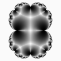
棋盤
目標集（臨界前點）

Numerical approximation of Julia set for fc(z)= z^2 + c 
child_period  = 3 
internal argument in turns = 1 / 3
parameter c = -0.1250000000000000 +0.6495190528383290*I 
fixed point alfa z = a = -0.2500000000000000 +0.4330127018922194*I 
external angles of rays landing on the fixed point  : t = 1/7 	t = 2/7 	t = 4/7
critical point z = zcr = 0.0000000000000000 +0.0000000000000000*I 
precritical point z = z_precritical = -0.2299551351162811 -0.1413579816050052*I  
external argument in turns of first ray landing on fixed point = 1 / 7

1/4

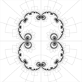
外部和內部的BDM

Julia set for fc(z)= z^2 + c 
internal argument in turns = 1/4
parameter c = 0.2500000000000000 +0.5000000000000000*I 
fixed point alfa z = a = 0.0000000000000000 +0.5000000000000000*I 
critical point z = zcr = 0.0000000000000000 +0.0000000000000000*I 
precritical point z = z_precritical = -0.2288905993372869 -0.0151096456992677*I  
external angles of rays landing on fixed point: 1/15, 2/15, 4/15, 8/15 ( in turns)

5/11

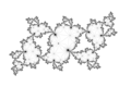
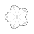
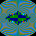
外部射線和臨界軌道（11臂星）

Numerical approximation of Julia set for fc(z)= z^2 + c 
parameter c = ( -0.6900598700150440 ; 0.2760264827846140 ) 
fixed point alfa z = a = ( -0.4797464868072486 ; 0.1408662784207147 ) 
external angle of ray landing on fixed point: 341/2047

另請參閱

拋物擾動
使用者:Tamfang 的雙曲鑲嵌中的棋盤：圖片和 Python 程式碼
https://plus.google.com/110803890168343196795/posts/Eun6pZVkkmA
shadertoy: Orbit trapped julia 由 maeln 於 2016 年 1 月 19 日建立
etale_cohomology 的全純棋盤
花椰菜的萼片
維基百科：計算機圖形學中的斑馬條紋
真實樹逼近花椰菜：收斂到花椰菜朱利亞集的樹。頂點集與 z 平方加四分之一的臨界點的廣義軌道一一對應。^[11]

參考文獻

[1] Arnaud Cheritat 的單奇異全純對映的近拋物重整化

[2] Arnaud Cheritat 關於 Inou 和 Shishikura 的近拋物重整化

[3] Mitsuhiro Shishikura 的近拋物重整化的應用

[4] Robert L. Devaney 的複雜動力系統，第

[5] Sabyasachi Mukherjee 的反全純動力學：引數空間的拓撲和拉直的不連續性

[6] T Kawahira 的瓷磚

[7] A Cheritat 的棋盤

[8] s:Category:用 Mandel 建立的分形

[9] Wolf Jung 的 Mandel 程式

[10] Wolf Jung 的 Mandel 程式

[11] Oleg Ivrii（特拉維夫大學），“樹的形狀”

[1]

[2]

[3]

[4]

[5]

[6]

[7]

[8]

[9]

[10]

[11]