動力學

實解析單峰動力學^[1]

圖表型別

二維圖表

引數是水平軸上的變數
- 分岔圖 : P-曲線（=週期點）與引數的關係^[2]
- 軌道圖 : 臨界軌道的點與引數的關係
- 骨架圖（臨界曲線 = q-曲線)^[3]
- 李雅普諾夫圖 : 李雅普諾夫指數與引數的關係^[4]
- 倍增圖 : 週期軌道的倍增因子與引數的關係
常數引數圖
- 蛛網圖或 Verhulst 圖 ^[5] = 圖形迭代
- 迭代與時間圖^[6] = 連線的散點圖 = 時間序列
- 不變密度圖、直方圖，^[7] 軌道的分佈，^[8] 頻率分佈 ^[9] = 功率譜 ^[10]
- 龐加萊圖^[11]^[12]

軌道圖
臨界曲線
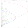實二次對映的分岔圖。顯示了週期為 1、2、4 和 8 的週期點
軌道圖和李雅普諾夫圖
倍增圖
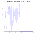
邏輯斯諦對映蛛網圖和時間演化 a=3.2

變換

指數變換引數軸

標準水平軸
變換後的水平軸以顯示倍週期級聯
3 個視窗，具有非線性，即對數 x 軸刻度

三維圖表

動畫的蛛網圖
動畫的連線散點圖

對映

由於數值誤差，同一個方程的不同實現可能會給出不同的軌跡。例如：r*x*(1-x) 和 r*x - r*x*x
對初始條件的敏感性：“初始條件的微小差異會導致系統長期行為的巨大差異。這種屬性有時被稱為‘蝴蝶效應’。”^[13]

對映型別

倍增對映

帳篷對映

帳篷對映的軌道

雙精度計算和數值誤差
提高精度，無誤差

邏輯斯諦對映

名稱

邏輯斯諦對映 ^[14]: $f(x)=rx(1-x),$ ^[15]
邏輯斯諦方程 $x_{n+1}=f(x_{n}),$
邏輯斯諦差分方程 $x_{n+1}=rx_{n}(1-x_{n}),$
離散動力系統

邏輯斯諦對映^[16]^[17] 由一個遞推關係（差分方程）定義

x_{n+1}=rx_{n}(1-x_{n}),

其中

$r$ 是一個給定的常數引數
$x_{0}$ 是給定的初始項
$x_{n}$ 是由該關係確定的後續項

不要與

微分方程（給出連續版本）混淆

Bash 程式碼 ^[18] Khan Academy 的 Javascript 程式碼 ^[19] MATLAB 程式碼

r_values = (2:0.0002:4)';
iterations_per_value = 10;
y = zeros(length(r_values), iterations_per_value);
y0 = 0.5;
y(:,1) = r_values.*y0*(1-y0);
for i = 1:iterations_per_value-1
    y(:,i+1) = r_values.*y(:,i).*(1-y(:,i));
end
plot(r_values, y, '.', 'MarkerSize', 1);
grid on;

另見 Lasin ^[20]

Maxima CAS 程式碼 ^[21]

/* Logistic diagram by Mario Rodriguez Riotorto using Maxima CAS draw packag  */
pts:[];
for r:2.5 while r <= 4.0 step 0.001 do /* min r = 1 */
		(x: 0.25,
		for k:1 thru 1000 do x: r * x * (1-x), /* to remove points from image compute and do not draw it */
		for k:1 thru 500  do (x: r * x * (1-x), /* compute and draw it */
        	 	 pts: cons([r,x], pts))); /* save points to draw it later, re=r, im=x */
load(draw);
draw2d(	terminal   = 'png,
	file_name = "v",
        dimensions = [1900,1300],
	title      = "Bifurcation diagram, x[i+1] = r*x[i]*(1 - x[i])",
	point_type = filled_circle,
	point_size = 0.2,
	color = black,
	points(pts));

顯式解

當 r=4 時，該系統對第 n 次迭代有顯式解 :^[22]

  $x_{n}=sin^{2}(2^{n}arcsin{\sqrt {x_{0}}})$

精度

混沌狀態下的數值精度："必須指定的精度位數約為迭代次數的 0.6 倍。因此，為了確定 is x10 000，我們需要約 6000 位數字。"

"因此，在混沌狀態下，不可能預測 xn 在非常大的 n 的值。" ^[23]

更好的影像

為了顯示更多細節，請使用提示，由使用者：PAR 提供。

"橫軸是 r 引數，縱軸是 x 變數。該影像是透過形成一個 1601 x 1001 陣列建立的，該陣列表示 r 和 x 的 0.001 增量。使用 x=0.25 的起始值，並將對映迭代 1000 次以穩定 x 值。然後計算了每個 r 值的 100,000 個 x 值，並且對於每個 x 值，影像中相應的 (x,r) 畫素加 1。然後將每一列（對應於特定 r 值）中的所有值乘以該列中非零畫素的數量，以使強度均勻。將超過 250,000 的值設定為 250,000，然後將整個影像歸一化為 0-255。最後，將 r 值低於 3.57 的畫素變暗以提高可見度。"

另見

來自 learner.org 的提示 ^[24]

   "The "problem" with pretty much all fractal-type systems, is, that, what happens at the beginning of an actually infinite iterational scheme, is often not descriptive of the long-time limit behaviour. And that's happening with the perturbed Lyapunov exponent from Mario Markus' algorithm as well. If I recall correctly, he states in his 90's article something like "let the x-value settle in". It's similar to the statement "for sufficiently large N" in math papers or in general with convergent series.
   The actual value of how many skipping iterations one performs, is, however, (at least afaik) just a guess till you're satisfied with the quality of the image. In my images, I could not get rid of those artifacts in full, one example being the UFO image, where vasyan did a great job removing those spots:
   vasyan's: https://fractalforums.org/index.php?action=gallery;sa=view;id=2388
   my version (with spots): https://fractalforums.org/index.php?action=gallery;sa=view;id=1960" marcm200^[25]

李雅普諾夫指數

Matlab 中的程式碼 ^[26]
G. Pastor, M. Romera 和 F. Montoya，“一維二次對映中李雅普諾夫指數的修正”，Physica D，107 (1997)，17-22。預印本

不變測度

狀態空間中的不變測度或機率密度 ^[27]

YouTube 上的影片 ^[28]

實二次對映

Chip Ross 提供的精彩影像 ^[29]

對於 $x_{n+1}=x_{n}^{2}-c$ ，MATLAB 中的程式碼可以寫成

c = (0:0.001:2)';
iterations_per_value = 100;
y = zeros(length(c), iterations_per_value);
y0 = 0;
y(:,1) = y0.^2 - c;
for i = 1:iterations_per_value-1
    y(:,i+1) = y(:,i).^2 - c;
end
plot(c, y, '.', 'MarkerSize', 1, 'MarkerEdgeColor', 'black');

用於繪製實二次對映的 Maxima CAS 程式碼： $f_{c}(z)=z^{2}+c$

/* based on the code by by Mario Rodriguez Riotorto */
pts:[];
for c:-2.0 while c <= 0.25 step 0.001 do 
                (x: 0.0,
                for k:1 thru 1000 do x: x * x+c, /* to remove points from image compute and do not draw it */
                for k:1 thru 500  do (x:  x * x+c, /* compute and draw it */
                         pts: cons([c,x], pts))); /* save points to draw it later, re=r, im=x */
load(draw);
draw2d( terminal   = 'svg,
        file_name = "b",
        dimensions = [1900,1300],
        title      = "Bifurcation diagram, x[i+1] = x[i]*x[i] +c",
        point_type = filled_circle,
        point_size = 0.2,
        color = black,
        points(pts));

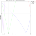
李雅普諾夫指數

program lapunow;

  { program draws bifurcation diagram y[n+1]=y[n]*y[n]+x,} { blue}
  {  x: -2 < x < 0.25 }
  {  y: -2 < y < 2    }
  {  and Lyapunov exponet for each x { white}

  uses crt,graph,
        { modul niestandardowy }
       bmpM, {screenCopy}
       Grafm;
  var xe,xemax,xe0,yemax,i1,i2:integer;
      yer,y,x,w,dx,lap:real;

  const xmin=-2;         { wspolczynnik   funkcji fx(y) }
        xmax=0.25;
        ymax=2;
        ymin=-2;
        i1max=100;            { liczba iteracji }
        i2max=20;
        lapmax=10;
        lapmin=-10;

   function wielomian2st(y,x:real) :real;
     begin
       wielomian2st:=y*y+x;
     end;  { wielomian2st }

  procedure wstep;
     begin
       opengraf;
       randomize;            { przygotowanie generatora liczb losowych }
       xemax:=getmaxx;              { liczba pixeli }
       yemax:=getmaxy;
       w:=(yemax+1)/(ymax-ymin);
       dx:=(xmax-xmin)/(xemax+1);
     end;

  begin {cialo}
    wstep;
    for xe:=xemax downTo 0 do
      begin {xe}
        x:=xmin+xe*dx;     { liniowe skalowanie x=a*xe+b }
        i1:=0;
        i2:=0;
        lap:=0;
        y:=random;        { losowy wybor    y0 : 0<y0<1 }

        while (abs(y)<ymax) and (i1<i1max)
        do
          begin {while i1}
            y:=wielomian2st(y,x);
            i1:=i1+1;
            lap:=lap+ln(abs(2*y)+0.1);
            if keypressed then halt;
          end; {while i1}

        while (i2<i2max) and (abs(y)<ymax)
         do
          begin   {while i2}
            y:=wielomian2st(y,x);
            yer:=(y-ymin)*w;         { skalowanie }
            putpixel(xe,yemax-round(yer),blue); { diagram bifurkacyjny }
            i2:=i2+1;
            lap:=lap+ln(abs(2*y)+0.1);
            if keypressed then halt;
          end; {while i2}

          lap:=lap/(i1max+i2max);
          yer:=(lap-lapmin)*(yemax+1)/(lapmax-lapmin);
          putpixel(xe,yemax-round(yer),white);         { wsp Lapunowa }
          putpixel(xe,yemax-round(-ymin*w),red);       { y=0 }
          putpixel(xe,yemax-round((1-ymin)*w),green);  { y=1}

      end; {xe}

    {..... os 0Y .......................................................}
    setcolor(red);
    xe0:=round((0-Xmin)/dx);     {xe0= xe : x=0 }
    line(xe0,0,xe0,yemax);
     SetColor(red);
    OutTextXY(XeMax-50,yemax-round((0-ymin)*w)+10,'y=0 ');
    SetColor(blue);
    OutTextXY(XeMax-50,yemax-round((1-ymin)*w)+10,'y=1');
    {....................................................................}
    screenCopy('screen',640,480);
    {}
    repeat until keypressed;
    closegraph;

 end.

{ Adam Majewski
Turbo Pascal 7.0  Borland
 MS-Dos / Microsoft}

縮放

分形論壇：渲染分岔圖

週期

張成的多項式對映的 n 週期和論文：邏輯斯諦對映的週期

點

常數

維基百科中的費根鮑姆常數

屬性

自相似性、縮放和重整化

邏輯斯諦對映的費根鮑姆縮放定律^[30]

另請參閱

軟體

影片

參考文獻

[1] 單峰動力學 40 年：紀念 Artur Avila 贏得 Brin 獎，作者：Mikhail Lyubich

[2] 分岔與軌道圖，作者：Chip Ross

[3] th.stackexchange 問題：分岔圖上的線是什麼？

[4] 一維二次對映中 Lyapunov 指數的修正，作者：Gerardo Pastor、Miguel Romera、Fausto Montoya Vitini。《非線性現象物理 D》，107(1):17 · 1997 年 8 月

[5] 維基百科：蛛網圖

[6] 一維動力系統第 3 部分：迭代，作者：Hinke Osinga

[7] 維基百科：直方圖

[8] 混沌理論：對引數 R 的依賴性

[9] 蝙蝠國，作者：xian

[10] 邏輯斯諦對映的功率譜，來自 Wolfram Mathematica

[11] 維基百科：龐加萊對映

[12] ysics.stackexchange 問題：龐加萊平面和邏輯斯諦對映

[13] 邏輯斯諦方程，作者：Didier Gonze

[May,_Robert_M_1976-14] May, Robert M. (1976). "Simple mathematical models with very complicated dynamics". Nature. 261 (5560): 459–467. Bibcode:1976Natur.261..459M. doi:10.1038/261459a0. hdl:10338.dmlcz/104555. PMID 934280.

[15] 具有非常複雜動力學的簡單數學模型，作者：R May

[16] 邏輯斯諦對映與混沌，作者：Elmer G. Wiens

[17] Ausloos，Marcel，Dirickx，Michel（編）：邏輯斯諦對映與通往混沌的道路

[18] 邏輯斯諦對映，作者：M.R. Titchener

[19] 可汗學院：邏輯斯諦對映

[20] Lasin - Matlab 程式碼

[21] 邏輯斯諦圖，作者：Mario Rodriguez Riotorto，使用 Maxima CAS draw 包繪製

[22] 邏輯斯諦對映中的雙精度誤差：統計研究與動力學解釋，作者：J. A. Oteo、J. Ros

[23] 邏輯斯諦對映，作者：A. Peter Young

[24] rner.org 教材

[25] ractalforums.org：我的 Lyapunov 分形渲染中可能出現哪些瑕疵

[26] 計算邏輯斯諦對映的 Lyapunov 指數 - LASIN

[27] 不變測度練習，作者：James P. Sethna、Christopher R. Myers

[28] 邏輯斯諦對映的不變測度，作者：todo314

[29] Chip Ross：分岔與軌道圖

[30] 沃爾弗拉姆演示：Logistic 地圖的費根鮑姆標度定律

[1]

[2]

[3]

[4]

[5]

[6]

[7]

[8]

[9]

[10]

[11]

[12]

[13]

[14]

[15]

[16]

[17]

[18]

[19]

[20]

[21]

[22]

[23]

[24]

[25]

[26]

[27]

[28]

[29]

[30]