平面的座標
一般型別
線性/非線性(軸的刻度)
維度:1D、2D、3D、...
3D 的方向手性(右手座標系 (RHS) 或左手座標系 (LHS))[ 1]
原點位置左上角原點座標系(原點位於螢幕的左上角,x 和 y 向右和向下為正)
左下角原點座標系(原點位於視窗或客戶端區域的左下角)
中間 = 中心原點座標系(0,0 座標位於中間。x 從左到右增加。y 從下到上增加。)
[ 2]
笛卡爾座標系(直角、正交)
橢圓座標系(曲線座標)
拋物線
極座標
對數極座標
雙極座標
規範化齊次座標 計算機圖形中的型別
這兩種型別之間的關係建立了新專案
畫素[ 5]
螢幕和整數座標之間的對映(轉換)[ 6] [ 7]
裁剪
光柵化
地理空間座標地理座標系 (GCS)
空間參考系統 (SRS) 或座標參考系統 (CRS) 笛卡爾座標系用於歐幾里得幾何。
笛卡爾座標系
1D、2D、3D、...
每個軸上的線性刻度(保持形狀)
座標 元素
原點 (0,0) 及其位置
單位
方向
寬度、高度 齊次座標或射影座標,由奧古斯特·費迪南德·莫比烏斯於 1827 年引入,是射影幾何中使用的一種座標系。
有理貝塞爾曲線 - 在齊次座標中定義的多項式曲線(藍色)及其在平面上的投影 - 有理曲線(紅色) 它們具有以下優點:
可以使用有限座標表示包括無窮遠點在內的點的座標
涉及齊次座標的公式通常比它們的笛卡爾對應公式更簡單、更對稱
齊次座標具有廣泛的應用,包括計算機圖形和三維計算機視覺,它們允許仿射變換以及一般來說射影變換很容易用矩陣表示
使用規範化的齊次座標避免了有理函式迭代中的溢位和下溢錯誤 迭代 在齊次座標中,二維平面上的一個點是一個三元組(一個由 3 個數字組成的有限有序列表(序列))[ 8] x , y , w {\displaystyle x,y,w}
從齊次座標 ( x , y , w ) {\displaystyle (x,y,w)} ( x , y ) {\displaystyle (x,y)} x {\displaystyle x} y {\displaystyle y} w {\displaystyle w} [ 9]
        (


            x
            w


        ,


            y
            w


        )


    {\displaystyle ({\frac {x}{w}},{\frac {y}{w}})}
( x , y ) {\displaystyle (x,y)}
        (
        x
        ,
        y
        ,
        1
        )


    {\displaystyle (x,y,1)}
二維卷積動畫 在數學中,對數極座標 (或對數極座標 )是二維座標系,其中點由兩個數字標識
對數極座標與極座標密切相關,極座標通常用於描述具有某種旋轉對稱性的平面域。在諸如調和分析和複分析的領域中,對數極座標比極座標更規範。另請參閱 指數對映
平面上的對數極座標 由一對實數 (ρ,θ) 組成,其中 ρ 是給定點與原點之間距離的對數,θ 是參考線(x 軸)與過原點和該點的直線之間的角度。角度座標與極座標相同,而半徑座標根據以下規則進行變換
r = e ρ {\displaystyle r=e^{\rho }} 其中 r {\displaystyle r}
對數極座標對映 :從笛卡爾空間 (x,y) 到極座標空間或 (ρ,θ) 空間的近似對映[ 10]
        x
        ,
        y
        →
        ρ
        ,
        θ
        →
        l
        o
        g
        (
        ρ
        )
        ,
        θ


    {\displaystyle x,y\to \rho ,\theta \to log(\rho ),\theta }
        ρ
        =


            (
            x
            −

              x

                c


              )

                2


            +
            (
            y
            −

              y

                c


              )

                2


    {\displaystyle \rho ={\sqrt {(x-x_{c})^{2}+(y-y_{c})^{2}}}}


        θ
        =


              y
              −

                y

                  c


              x
              −

                x

                  c


    {\displaystyle \theta ={\frac {y-y_{c}}{x-x_{c}}}}
其中
其中 ρ {\displaystyle \rho } ( x c , y c ) {\displaystyle (x_{c},y_{c})}
θ {\displaystyle \theta } 早在 1970 年代末,離散螺旋座標系的應用已出現在影像分析(影像配準)中。用這種座標系而不是笛卡爾座標系來表示影像,在旋轉或放大影像時具有計算優勢。此外,人眼視網膜中的光感受器分佈方式與螺旋座標系非常相似。[ 11]
對數極座標還可以用於構建拉東變換及其逆變換的快速方法。[ 12]
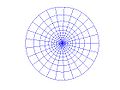
為了用數值方法求解一個域中的偏微分方程,必須在這個域中引入一個離散的座標系。如果這個域具有旋轉對稱性,並且您想要一個由矩形組成的網格,那麼極座標是一個糟糕的選擇,因為它在圓心處會產生三角形而不是矩形。
然而,可以透過以下方式引入對數極座標來解決這個問題
將平面分成邊長為 2 π {\displaystyle \pi } n 的正方形網格,其中 n 是一個正整數
使用復指數函式在平面上建立對數極座標網格。然後,左半平面被對映到單位圓盤上,半徑的數量等於 n 。更重要的是,可以將這些正方形的對角線對映到單位圓盤上,這將在單位圓盤中產生一個由螺旋線組成的離散座標系,請參閱右側的圖形。 影像中的座標值始終為正[ 13]
原點 = 點 (90, 0) 位於螢幕的左上角
座標是整數值
螢幕上的座標系是左手系的,即 x 座標從左到右增加,y 座標從上到下增加。 柵格 2D 圖形
// from screen to world coordinate ; linear mapping
// uses global cons
double GiveZx ( int ix )
{
return ( ZxMin + ix * PixelWidth );
}
// uses globaal cons
double GiveZy ( int iy )
{
return ( ZyMax - iy * PixelHeight );
} // reverse y axis
complex double GiveZ ( int ix , int iy )
{
double Zx = GiveZx ( ix );
double Zy = GiveZy ( iy );
return Zx + Zy * I ;
}
// modified code using center and radius to scan the plane
int height = 720 ;
int width = 1280 ;
double dWidth ;
double dRadius = 1.5 ;
double complex center = -0.75 * I ;
double complex c ;
int i , j ;
double width2 ; // = width/2.0
double height2 ; // = height/2.0
width2 = width / 2.0 ;
height2 = height / 2.0 ;
complex double coordinate ( int i , int j , int width , int height , complex double center , double radius ) {
double x = ( i - width / 2.0 ) / ( height / 2.0 );
double y = ( j - height / 2.0 ) / ( height / 2.0 );
complex double c = center + radius * ( x - I * y );
return c ;
}
for ( j = 0 ; j < height ; ++ j ) {
for ( i = 0 ; i < width ; ++ i ) {
c = coordinate ( i , j , width , height , center , dRadius );
// do smth
}
}
double pixel_spacing = radius / ( height / 2.0 );
complex double c = center + pixel_spacing * ( x - width / 2.0 + I * ( y - height / 2.0 ));
另請參閱
通常,存在許多不同的座標系來描述幾何圖形。不同系統之間的關係由座標變換 描述,該變換給出了一個系統中的座標關於另一個系統中的座標的公式。例如,在平面上,如果笛卡爾座標 (x , y ) 和極座標 (r , θ ) 具有相同的原點,並且極軸是正的 x 軸,則從極座標到笛卡爾座標的座標變換由 x = r cosθ 和 y = r sinθ 給出。
對於空間到自身的每個雙射,都可以關聯兩個座標變換
使得每個點的像的新座標與原始點的老座標相同(對映的公式是座標變換的逆公式)
使得每個點的像的老座標與原始點的新座標相同(對映的公式與座標變換的公式相同) 例如,在 1D 中,如果對映是向右平移 3,則第一個將原點從 0 移動到 3,使得每個點的座標減少 3,而第二個將原點從 0 移動到 -3,使得每個點的座標增加 3。以下是使用最廣泛的一些座標變換的列表。
設 (x , y ) 為標準笛卡爾座標,(r , θ ) 為標準極座標。
x = r cos θ y = r sin θ ∂ ( x , y ) ∂ ( r , θ ) = [ cos θ − r sin θ sin θ r cos θ ] Jacobian = det ∂ ( x , y ) ∂ ( r , θ ) = r {\displaystyle {\begin{aligned}x&=r\cos \theta \\y&=r\sin \theta \\[5pt]{\frac {\partial (x,y)}{\partial (r,\theta )}}&={\begin{bmatrix}\cos \theta &-r\sin \theta \\\sin \theta &r\cos \theta \end{bmatrix}}\\[5pt]{\text{Jacobian}}=\det {\frac {\partial (x,y)}{\partial (r,\theta )}}&=r\end{aligned}}} 從笛卡爾座標到對數極座標的變換公式由下式給出
{ ρ = ln ( x 2 + y 2 ) , θ = atan2 ( y , x ) . {\displaystyle {\begin{cases}\rho =\ln \left({\sqrt {x^{2}+y^{2}}}\right),\\\theta =\operatorname {atan2} (y,\,x).\end{cases}}} 從對數極座標到笛卡爾座標的變換公式為
{ x = e ρ cos θ , y = e ρ sin θ . {\displaystyle {\begin{cases}x=e^{\rho }\cos \theta ,\\y=e^{\rho }\sin \theta .\end{cases}}} 使用複數 (x , y ) = x + iy ,後一種變換可以寫成
x + i y = e ρ + i θ {\displaystyle x+iy=e^{\rho +i\theta }} 即復指數函式。
由此可以得出,諧波分析和複分析中的基本方程將與笛卡爾座標系中的形式相同。這在極座標系中是不成立的。
x = e ρ cos θ , y = e ρ sin θ . {\displaystyle {\begin{aligned}x&=e^{\rho }\cos \theta ,\\y&=e^{\rho }\sin \theta .\end{aligned}}} 使用複數 ( x , y ) = x + i y ′ {\displaystyle (x,y)=x+iy'}
x + i y = e ρ + i θ {\displaystyle x+iy=e^{\rho +i\theta }} 也就是說,它是用復指數函式給出的。
x = a sinh τ cosh τ − cos σ y = a sin σ cosh τ − cos σ {\displaystyle {\begin{aligned}x&=a{\frac {\sinh \tau }{\cosh \tau -\cos \sigma }}\\y&=a{\frac {\sin \sigma }{\cosh \tau -\cos \sigma }}\end{aligned}}} x = 1 4 c ( r 1 2 − r 2 2 ) y = ± 1 4 c 16 c 2 r 1 2 − ( r 1 2 − r 2 2 + 4 c 2 ) 2 {\displaystyle {\begin{aligned}x&={\frac {1}{4c}}\left(r_{1}^{2}-r_{2}^{2}\right)\\y&=\pm {\frac {1}{4c}}{\sqrt {16c^{2}r_{1}^{2}-(r_{1}^{2}-r_{2}^{2}+4c^{2})^{2}}}\end{aligned}}} x = ∫ cos [ ∫ κ ( s ) d s ] d s y = ∫ sin [ ∫ κ ( s ) d s ] d s {\displaystyle {\begin{aligned}x&=\int \cos \left[\int \kappa (s)\,ds\right]ds\\y&=\int \sin \left[\int \kappa (s)\,ds\right]ds\end{aligned}}} r = x 2 + y 2 θ ′ = arctan | y x | {\displaystyle {\begin{aligned}r&={\sqrt {x^{2}+y^{2}}}\\\theta '&=\arctan \left|{\frac {y}{x}}\right|\end{aligned}}} 注意:求解 θ ′ {\displaystyle \theta '} 0 < θ < π 2 {\textstyle 0<\theta <{\frac {\pi }{2}}} θ {\displaystyle \theta } θ {\displaystyle \theta } θ {\displaystyle \theta }
對於 θ ′ {\displaystyle \theta '} θ = θ ′ {\displaystyle \theta =\theta '}
對於 θ ′ {\displaystyle \theta '} θ = π − θ ′ {\displaystyle \theta =\pi -\theta '}
對於 θ ′ {\displaystyle \theta '} θ = π + θ ′ {\displaystyle \theta =\pi +\theta '}
對於 θ ′ {\displaystyle \theta '} θ = 2 π − θ ′ {\displaystyle \theta =2\pi -\theta '} 必須用這種方式求解 θ {\displaystyle \theta } θ {\displaystyle \theta } tan θ {\displaystyle \tan \theta } − π 2 < θ < + π 2 {\textstyle -{\frac {\pi }{2}}<\theta <+{\frac {\pi }{2}}} π {\displaystyle \pi }
注意,也可以使用
r = x 2 + y 2 θ ′ = 2 arctan y x + r {\displaystyle {\begin{aligned}r&={\sqrt {x^{2}+y^{2}}}\\\theta '&=2\arctan {\frac {y}{x+r}}\end{aligned}}} r = r 1 2 + r 2 2 − 2 c 2 2 θ = arctan [ 8 c 2 ( r 1 2 + r 2 2 − 2 c 2 ) r 1 2 − r 2 2 − 1 ] {\displaystyle {\begin{aligned}r&={\sqrt {\frac {r_{1}^{2}+r_{2}^{2}-2c^{2}}{2}}}\\\theta &=\arctan \left[{\sqrt {{\frac {8c^{2}(r_{1}^{2}+r_{2}^{2}-2c^{2})}{r_{1}^{2}-r_{2}^{2}}}-1}}\right]\end{aligned}}} 其中,2c 表示兩極之間的距離。
ρ = log x 2 + y 2 , θ = arctan y x . {\displaystyle {\begin{aligned}\rho &=\log {\sqrt {x^{2}+y^{2}}},\\\theta &=\arctan {\frac {y}{x}}.\end{aligned}}} κ = x ′ y ″ − y ′ x ″ ( x ′ 2 + y ′ 2 ) 3 2 s = ∫ a t x ′ 2 + y ′ 2 d t {\displaystyle {\begin{aligned}\kappa &={\frac {x'y''-y'x''}{({x'}^{2}+{y'}^{2})^{\frac {3}{2}}}}\\s&=\int _{a}^{t}{\sqrt {{x'}^{2}+{y'}^{2}}}\,dt\end{aligned}}} κ = r 2 + 2 r ′ 2 − r r ″ ( r 2 + r ′ 2 ) 3 2 s = ∫ a φ r 2 + r ′ 2 d φ {\displaystyle {\begin{aligned}\kappa &={\frac {r^{2}+2{r'}^{2}-rr''}{(r^{2}+{r'}^{2})^{\frac {3}{2}}}}\\s&=\int _{a}^{\varphi }{\sqrt {r^{2}+{r'}^{2}}}\,d\varphi \end{aligned}}} 設 (x, y, z) 為標準笛卡爾座標,(ρ, θ, φ) 為 球面座標 ,其中 θ 為從 +Z 軸測量的角度(如 [1] ,參見 球面座標 中的約定)。由於 φ 的範圍為 360°,因此在取 φ 的反正切時,與極座標(二維)座標系中的情況相同。θ 的範圍為 180°,從 0° 到 180°,在從反餘弦計算時不會出現任何問題,但在取反正切時要小心。
如果在另一種定義中,選擇 θ 從 −90° 到 +90°,與先前定義的方向相反,則可以從反正弦唯一地找到它,但要小心反餘切。在這種情況下,下面所有公式中 θ 中的所有引數都應該交換正弦和餘弦,並且作為導數也應該交換加號和減號。
所有除以零的結果都是沿一個主軸方向的特殊情況,實際上最容易透過觀察解決。
x = ρ sin θ cos φ y = ρ sin θ sin φ z = ρ cos θ ∂ ( x , y , z ) ∂ ( ρ , θ , φ ) = ( sin θ cos φ ρ cos θ cos φ − ρ sin θ sin φ sin θ sin φ ρ cos θ sin φ ρ sin θ cos φ cos θ − ρ sin θ 0 ) {\displaystyle {\begin{aligned}x&=\rho \,\sin \theta \,\cos \varphi \\y&=\rho \,\sin \theta \,\sin \varphi \\z&=\rho \,\cos \theta \\{\frac {\partial (x,y,z)}{\partial (\rho ,\theta ,\varphi )}}&={\begin{pmatrix}\sin \theta \cos \varphi &\rho \cos \theta \cos \varphi &-\rho \sin \theta \sin \varphi \\\sin \theta \sin \varphi &\rho \cos \theta \sin \varphi &\rho \sin \theta \cos \varphi \\\cos \theta &-\rho \sin \theta &0\end{pmatrix}}\end{aligned}}} 因此體積元
d x d y d z = det ∂ ( x , y , z ) ∂ ( ρ , θ , φ ) d ρ d θ d φ = ρ 2 sin θ d ρ d θ d φ {\displaystyle dx\;dy\;dz=\det {\frac {\partial (x,y,z)}{\partial (\rho ,\theta ,\varphi )}}d\rho \;d\theta \;d\varphi =\rho ^{2}\sin \theta \;d\rho \;d\theta \;d\varphi } x = r cos θ y = r sin θ z = z ∂ ( x , y , z ) ∂ ( r , θ , z ) = ( cos θ − r sin θ 0 sin θ r cos θ 0 0 0 1 ) {\displaystyle {\begin{aligned}x&=r\,\cos \theta \\y&=r\,\sin \theta \\z&=z\,\\{\frac {\partial (x,y,z)}{\partial (r,\theta ,z)}}&={\begin{pmatrix}\cos \theta &-r\sin \theta &0\\\sin \theta &r\cos \theta &0\\0&0&1\end{pmatrix}}\end{aligned}}} 因此體積元
d V = d x d y d z = det ∂ ( x , y , z ) ∂ ( r , θ , z ) d r d θ d z = r d r d θ d z {\displaystyle dV=dx\;dy\;dz=\det {\frac {\partial (x,y,z)}{\partial (r,\theta ,z)}}dr\;d\theta \;dz=r\;dr\;d\theta \;dz} ρ = x 2 + y 2 + z 2 θ = arctan ( x 2 + y 2 z ) = arccos ( z x 2 + y 2 + z 2 ) φ = arctan ( y x ) = arccos ( x x 2 + y 2 ) = arcsin ( y x 2 + y 2 ) ∂ ( ρ , θ , φ ) ∂ ( x , y , z ) = ( x ρ y ρ z ρ x z ρ 2 x 2 + y 2 y z ρ 2 x 2 + y 2 − x 2 + y 2 ρ 2 − y x 2 + y 2 x x 2 + y 2 0 ) {\displaystyle {\begin{aligned}\rho &={\sqrt {x^{2}+y^{2}+z^{2}}}\\\theta &=\arctan \left({\frac {\sqrt {x^{2}+y^{2}}}{z}}\right)=\arccos \left({\frac {z}{\sqrt {x^{2}+y^{2}+z^{2}}}}\right)\\\varphi &=\arctan \left({\frac {y}{x}}\right)=\arccos \left({\frac {x}{\sqrt {x^{2}+y^{2}}}}\right)=\arcsin \left({\frac {y}{\sqrt {x^{2}+y^{2}}}}\right)\\{\frac {\partial \left(\rho ,\theta ,\varphi \right)}{\partial \left(x,y,z\right)}}&={\begin{pmatrix}{\frac {x}{\rho }}&{\frac {y}{\rho }}&{\frac {z}{\rho }}\\{\frac {xz}{\rho ^{2}{\sqrt {x^{2}+y^{2}}}}}&{\frac {yz}{\rho ^{2}{\sqrt {x^{2}+y^{2}}}}}&-{\frac {\sqrt {x^{2}+y^{2}}}{\rho ^{2}}}\\{\frac {-y}{x^{2}+y^{2}}}&{\frac {x}{x^{2}+y^{2}}}&0\\\end{pmatrix}}\end{aligned}}} 另請參閱有關atan2 的文章,瞭解如何優雅地處理一些邊緣情況。
因此對於元素
d ρ d θ d φ = det ∂ ( ρ , θ , φ ) ∂ ( x , y , z ) d x d y d z = 1 x 2 + y 2 x 2 + y 2 + z 2 d x d y d z {\displaystyle d\rho \ d\theta \ d\varphi =\det {\frac {\partial (\rho ,\theta ,\varphi )}{\partial (x,y,z)}}dx\ dy\ dz={\frac {1}{{\sqrt {x^{2}+y^{2}}}{\sqrt {x^{2}+y^{2}+z^{2}}}}}dx\ dy\ dz} ρ = r 2 + h 2 θ = arctan r h φ = φ ∂ ( ρ , θ , φ ) ∂ ( r , h , φ ) = ( r r 2 + h 2 h r 2 + h 2 0 h r 2 + h 2 − r r 2 + h 2 0 0 0 1 ) det ∂ ( ρ , θ , φ ) ∂ ( r , h , φ ) = 1 r 2 + h 2 {\displaystyle {\begin{aligned}\rho &={\sqrt {r^{2}+h^{2}}}\\\theta &=\arctan {\frac {r}{h}}\\\varphi &=\varphi \\{\frac {\partial (\rho ,\theta ,\varphi )}{\partial (r,h,\varphi )}}&={\begin{pmatrix}{\frac {r}{\sqrt {r^{2}+h^{2}}}}&{\frac {h}{\sqrt {r^{2}+h^{2}}}}&0\\{\frac {h}{r^{2}+h^{2}}}&{\frac {-r}{r^{2}+h^{2}}}&0\\0&0&1\\\end{pmatrix}}\\\det {\frac {\partial (\rho ,\theta ,\varphi )}{\partial (r,h,\varphi )}}&={\frac {1}{\sqrt {r^{2}+h^{2}}}}\end{aligned}}} r = x 2 + y 2 θ = arctan ( y x ) z = z {\displaystyle {\begin{aligned}r&={\sqrt {x^{2}+y^{2}}}\\\theta &=\arctan {\left({\frac {y}{x}}\right)}\\z&=z\quad \end{aligned}}} ∂ ( r , θ , h ) ∂ ( x , y , z ) = ( x x 2 + y 2 y x 2 + y 2 0 − y x 2 + y 2 x x 2 + y 2 0 0 0 1 ) {\displaystyle {\frac {\partial (r,\theta ,h)}{\partial (x,y,z)}}={\begin{pmatrix}{\frac {x}{\sqrt {x^{2}+y^{2}}}}&{\frac {y}{\sqrt {x^{2}+y^{2}}}}&0\\{\frac {-y}{x^{2}+y^{2}}}&{\frac {x}{x^{2}+y^{2}}}&0\\0&0&1\end{pmatrix}}} r = ρ sin φ h = ρ cos φ θ = θ ∂ ( r , h , θ ) ∂ ( ρ , φ , θ ) = ( sin φ ρ cos φ 0 cos φ − ρ sin φ 0 0 0 1 ) det ∂ ( r , h , θ ) ∂ ( ρ , φ , θ ) = − ρ {\displaystyle {\begin{aligned}r&=\rho \sin \varphi \\h&=\rho \cos \varphi \\\theta &=\theta \\{\frac {\partial (r,h,\theta )}{\partial (\rho ,\varphi ,\theta )}}&={\begin{pmatrix}\sin \varphi &\rho \cos \varphi &0\\\cos \varphi &-\rho \sin \varphi &0\\0&0&1\\\end{pmatrix}}\\\det {\frac {\partial (r,h,\theta )}{\partial (\rho ,\varphi ,\theta )}}&=-\rho \end{aligned}}} s = ∫ 0 t x ′ 2 + y ′ 2 + z ′ 2 d t κ = ( z ″ y ′ − y ″ z ′ ) 2 + ( x ″ z ′ − z ″ x ′ ) 2 + ( y ″ x ′ − x ″ y ′ ) 2 ( x ′ 2 + y ′ 2 + z ′ 2 ) 3 2 τ = x ‴ ( y ′ z ″ − y ″ z ′ ) + y ‴ ( x ″ z ′ − x ′ z ″ ) + z ‴ ( x ′ y ″ − x ″ y ′ ) ( x ′ y ″ − x ″ y ′ ) 2 + ( x ″ z ′ − x ′ z ″ ) 2 + ( y ′ z ″ − y ″ z ′ ) 2 {\displaystyle {\begin{aligned}s&=\int _{0}^{t}{\sqrt {{x'}^{2}+{y'}^{2}+{z'}^{2}}}\,dt\\[3pt]\kappa &={\frac {\sqrt {(z''y'-y''z')^{2}+(x''z'-z''x')^{2}+(y''x'-x''y')^{2}}}{({x'}^{2}+{y'}^{2}+{z'}^{2})^{\frac {3}{2}}}}\\[3pt]\tau &={\frac {x'''(y'z''-y''z')+y'''(x''z'-x'z'')+z'''(x'y''-x''y')}{{(x'y''-x''y')}^{2}+{(x''z'-x'z'')}^{2}+{(y'z''-y''z')}^{2}}}\end{aligned}}} wgpu 使用 D3D 和 Metal 的座標系:[ 14]
渲染:中心點為 0,半徑為 1,所以右上角為 (1,1),左下角為 (-1,-1)
紋理:0 為左上角點,右上角為 (1,0),左下角為 (0,1) [ 15]
是一個二維網格
x 從左到右增加:從 x=0 (最左邊) 到 x=+960 (最右邊)
y 從下到上遞減:從 y=+720 (底部) 到 y=0 (頂部).
原點 = 0,0 座標位於左上角 (畫布的左上角)
圖形管道的三個基本步驟
OpenGL 管道
圖形管道中的幾何步驟
3D 圖形渲染管道
OpenGL 中的五個不同的座標系:[ 16]
OpenGl
"OpenGL 在物件空間和世界空間中是右手座標系,但在視窗空間 (又稱螢幕空間) 中,我們突然變成了左手座標系"[ 17]
變換管道:區域性座標 -> 世界座標 -> 檢視座標 -> 剪下座標 -> 螢幕座標[ 18] [ 19]
使用齊次座標[ 20]
歸一化裝置座標 (NDC) 僅座標 (x,y,z) : -1 ≤ x,y,z ≤ +1。任何超出此範圍的座標都將被丟棄或剪下 = 不會在螢幕上顯示[ 21]
矩陣微積分 SVG 座標系
SVG 中的預設座標系與 HTML 中的座標系基本相同
畫布是所有 SVG 元素繪製的空間或區域[ 22]
視窗定義了一個繪製區域,該區域以大小 (寬度、高度) 和原點為特徵,以抽象使用者單位測量。術語 SVG 視窗不同於 CSS 中使用的“視窗”術語
視窗[ 23] 二維座標系[ 24]
↑ 約翰·T·貝爾博士的座標系 ↑ 維基百科:座標系 ↑ 計算機圖形學 StackExchange 問題:世界座標、觀察座標和裝置座標之間的區別是什麼 ↑ Javatpoint:計算機圖形學視窗 ↑ 畫素不是一個小方塊,由 Alvy Ray Smith 撰寫 ↑ 如何將世界座標轉換為螢幕座標,反之亦然 ↑ 如何在 OpenGL 中將二維世界座標轉換為螢幕座標 ↑ 文字和按鈕線上 - 一系列互動式內容的齊次座標互動式指南 ↑ 齊次座標,由 Yasen Hu 撰寫 ↑ 使用對數極座標變換和相位相關來恢復更高尺度的影像配準,JIGNESH NATVARLAL SARVAIYA、Suprava Patnaik 博士、Kajal Kothari,JPRR 第 7 卷,第 1 期(2012 年);doi:10.13176/11.355 ↑ Weiman、Chaikin,《用於影像處理和顯示的對數螺旋網格》,《計算機圖形學和影像處理》第 11 卷,第 197-226 頁(1979 年)。 ↑ Andersson、Fredrik,《使用對數極座標和部分反投影對 Radon 變換進行快速反演》,《SIAM 應用數學雜誌》第 65 卷,第 818-837 頁(2005 年)。 ↑ ronny restrepo:點雲座標 ↑ raphlinus:wgpu ↑ w3schools:畫布座標 ↑ learnopengl:座標系 ↑ stackoverflow 問題:OpenGL 座標系是左手系還是右手系 ↑ learnopengl:座標系 ↑ Paul Martz 撰寫的 OpenGL 變換管道 ↑ 宋浩安的齊次座標 ↑ 用於科學視覺化的 Python 和 OpenGL,版權所有 (c) 2018 - Nicolas P. Rougier ↑ ASPOSE 撰寫的 SVG 座標系和單位 ↑ Sara Soueidan 撰寫的 svg-coordinate-systems ↑ 二維座標系,倫敦大學金史密斯學院 

 裁剪
裁剪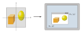 視窗-視口變換


 由對數極座標給出的圓盤中的離散座標系 (n = 25)
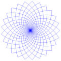 可以很容易地用對數極座標表示的圓盤中的離散座標系 (n = 25)
 顯示螺旋行為的曼德勃羅特分形的一部分


![{\displaystyle {\begin{aligned}x&=r\cos \theta \\y&=r\sin \theta \\[5pt]{\frac {\partial (x,y)}{\partial (r,\theta )}}&={\begin{bmatrix}\cos \theta &-r\sin \theta \\\sin \theta &r\cos \theta \end{bmatrix}}\\[5pt]{\text{Jacobian}}=\det {\frac {\partial (x,y)}{\partial (r,\theta )}}&=r\end{aligned}}}](https://wikimedia.org/api/rest_v1/media/math/render/svg/6e812d8ce26cec97482d277c012e638ee182d298)


![{\displaystyle {\begin{aligned}x&=\int \cos \left[\int \kappa (s)\,ds\right]ds\\y&=\int \sin \left[\int \kappa (s)\,ds\right]ds\end{aligned}}}](https://wikimedia.org/api/rest_v1/media/math/render/svg/0cf415cca15fe7faf409efdfa8323225993978f8)


![{\displaystyle {\begin{aligned}r&={\sqrt {\frac {r_{1}^{2}+r_{2}^{2}-2c^{2}}{2}}}\\\theta &=\arctan \left[{\sqrt {{\frac {8c^{2}(r_{1}^{2}+r_{2}^{2}-2c^{2})}{r_{1}^{2}-r_{2}^{2}}}-1}}\right]\end{aligned}}}](https://wikimedia.org/api/rest_v1/media/math/render/svg/40fd7b0ef6f1fea0e4467981685d16feb513186d)


![{\displaystyle {\begin{aligned}s&=\int _{0}^{t}{\sqrt {{x'}^{2}+{y'}^{2}+{z'}^{2}}}\,dt\\[3pt]\kappa &={\frac {\sqrt {(z''y'-y''z')^{2}+(x''z'-z''x')^{2}+(y''x'-x''y')^{2}}}{({x'}^{2}+{y'}^{2}+{z'}^{2})^{\frac {3}{2}}}}\\[3pt]\tau &={\frac {x'''(y'z''-y''z')+y'''(x''z'-x'z'')+z'''(x'y''-x''y')}{{(x'y''-x''y')}^{2}+{(x''z'-x'z'')}^{2}+{(y'z''-y''z')}^{2}}}\end{aligned}}}](https://wikimedia.org/api/rest_v1/media/math/render/svg/439b196b830ab79231f87b27a17af5ed4cf5f4e4)
 圖形管道的三個基本步驟
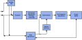 OpenGL 管道
 圖形管道中的幾何步驟
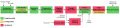 3D 圖形渲染管道
![[1]](https://commons.wikimedia.org/wiki/File:3D_Spherical.svg)