
分形/數學/向量場
向量場[1]
這裡主要描述了與時間無關的二維向量場的數值方法。
- 向量函式是一個給出向量作為輸出的函式
- 場:空間(平面,球體,...)
- 場線是一條始終與給定向量場相切的線
- 標量/向量/張量
- 標量是線上性代數中使用的實數。標量是零階張量
- 向量是一階張量。向量是標量的擴充套件
- 張量是向量的擴充套件
二維向量的形式:[2]
- [z1](當第一個點已知時,只有一個複數,例如 z0 是原點
- [z0, z1] = 兩個複數
- 4 個標量(實數)
- [x, y, dx , dy]
- [x0, y0, x1, y1]
- [x, y, 角度, 大小]
- 2 個標量:當第一個點已知時,[x1, y1] 用於第二個複數,例如 z0 是原點
函式的數值梯度
- "是一種使用已知函式在某些點的值來估計每個維度上偏導數的值的方法。"[3]
函式 f 在點 (x0,y0) 處的梯度函式 G
G(f,x0,y0) = (x1,y1)
輸入
- 函式 f
- 點 (x0,y0),計算梯度
輸出
- 從 (x0,yo) 到 (x1,y1) 的向量 = 梯度
見
計算:[4]
- "梯度計算為:(f(x + h) - f(x - h)) / (2*h),其中 h 是一個小的數字,通常為 1e-5,f(x) 將對每個輸入元素進行呼叫,並帶有 +h 和 -h 擾動。對於梯度檢查,建議使用 float64 型別以確保數值精度。"[5]
- 在 matlab 中[6][7]
- 在 R 中[8]
- python[9]
ODE means Ordinary Differential Equation, where "ordinary" means with derivative respect to only one variable (like ), as opposed to an equation with partial derivatives (like , , ...) called PDE. (matteo.basei)


分類標準
- 自治的 / 非自治的
- 與時間無關(= 穩定 = 穩態)或與時間相關(非穩態流)
- 維度:二維,三維,...
- 網格(網格)型別
- 標量函式
- 勢
- 力型別:電,磁,...
- 向量函式
- 方程(用於符號計算) - 常微分方程
- 數值(用於數值計算)
力型別 A 重力場
- 場線是 的解
- 測試質量的軌跡是 的解


其中
- g 是標準重力
- m 是質量
- F 是力場
電場
- 場線是點正電荷在電場作用下被迫移動時所遵循的路徑。由於靜止電荷引起的場線具有幾個重要特性,包括始終從正電荷起源並終止於負電荷,它們以直角進入所有良導體,並且它們從不交叉或自閉。 場線是一個代表性概念;場實際上滲透了線之間所有介於線之間的空間。根據需要代表場的精度,可以繪製更多或更少的線。對由靜止電荷產生的電場的研究稱為靜電學。
-
 靜電感應產生的導電物體(形狀)中感應電荷的示意圖,其中附近的電荷 (+) 的靜電場(帶箭頭的線)導致靜電感應
 -
 兩個相同導電球體在相反電勢下的電場


- Adrien Douady、Franiso Estrada 和 Pierrette Sentena。C 上的多項式向量場。未出版手稿
- Bodil Branner、Kealey Dias 編著的複數多項式向量場分類
- Kealey Dias、Lei Tan 編著的複數平面複數多項式向量場引數空間
- 從
- 平面(引數平面或動態平面)
- 標量函式
- 向量函式
- 使用標量函式(勢)建立標量場
- 使用向量函式(勢的梯度)從標量場建立向量場
- 計算
//https://editor.p5js.org/ndeji69/sketches/EA17R4HHa
// p5 js Tutorial】Swirling Pattern using Gradient for Generative Art by Nekodigi

//get gradient vector
function curl(x, y){
  var EPSILON = 0.001;//sampling interval
  //Find rate of change in X direction
  var n1 = noise(x + EPSILON, y);
  var n2 = noise(x - EPSILON, y);
  //Average to find approximate derivative
  var cx = (n1 - n2)/(2 * EPSILON);

  //Find rate of change in Y direction
  n1 = noise(x, y + EPSILON);
  n2 = noise(x, y - EPSILON);

  //Average to find approximate derivative
  var cy = (n1 - n2)/(2 * EPSILON);

  //return new createVector(cx, cy);//gradient toward higher position
  return new createVector(cy, -cx);//rotate 90deg
}

function draw() {
  tint(255, 4);
  image(noiseImg, 0, 0);//fill with transparent noise image
  //fill(0, 4);
  //rect(0, 0, width, height);

  strokeWeight(4);//particle size
  stroke(255);


  for(var i=0; i<particles.length; i++){
    var p = particles[i];//pick a particle
    p.pos.add(curl(p.pos.x/noiseScale, p.pos.y/noiseScale));
    point(p.pos.x, p.pos.y);
  }
}
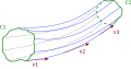
透過數值求解軌跡反向時間,可以清楚地看到分隔線。由於在求解正向時間軌跡時,軌跡會從分隔線發散,而在求解反向時間軌跡時,軌跡會收斂於分隔線。

- Aytan Hajiyeva Aytan Hajiyeva 2021 年 10 月 1 日編著的梯度下降
- Raghunath D Raghunath D 2019 年 1 月 28 日編著的梯度下降演算法
- SEBASTIAN RUDER 2016 年 1 月 19 日編著的梯度下降最佳化演算法概述 和 arxiv 上的 pdf 檔案
- Rong Ge • 2016 年 3 月 22 日編著的逃離鞍點
- Great Learning Team - 2020 年 5 月 24 日編著的機器學習中梯度下降的簡單指南
- Sagar Mainkar Sagar Mainkar 2018 年 8 月 25 日編著的 Python 中的梯度下降
問題陳述
- 場線追蹤(不是曲線素描[11]}
- 繪製等高線圖(在計算機圖形學中)= 數值延拓(在數學中)
- 在均勻網格(光柵掃描或畫素)上不分析其結構的情況下,從種子點透過向量場計算積分曲線
-
 自然引數延拓,是對迭代求解器到引數化問題的非常簡單的改編
 -
 單純形線性延拓演算法。
 -
 偽弧長延拓,基於這樣的觀察結果,即曲線的“理想”引數化是弧長,是曲線切空間中弧長的近似值\
 -


- 尤拉[14]
- RK2
- RK3
- RK4 - 這些取樣演算法的最初作者:Runge und Kutta。[15]
- 向量場尋路演算法如何工作?作者:PDN - PasDeNom
  None of these 4 methods generate an exact answer, but they are (from left to right) increasingly more accurate. They also take (from left to right) more and more time to finish as they require more samples for each iteration.
  You won't be able to create reliably closed curves using iterative sampling methods as small errors at any step may be amplified in successive steps. There is also no guarantee that the field-line ends up in the exact coordinate where it started.
  The Grasshopper metaball solver on the other hand uses a marching squares algorithm which is capable of finding closed loops because it is a grid-cell approach and sampling inaccuracy in one area doesn't carry over to another.
  However the solving of iso-curves is a very different process    from the solving of particle trajectories through fields. ...
  Typically field lines shoot to infinity rather than form closed loops. That is one reason why I chose the RK methods here, because marching-cubes is very bad at dealing with things that tend to infinity.[16]

給定一個向量場 和一個起點 ,可以透過迭代方式構建場線,方法是找到該點的場向量 。該點的單位切向量 為:。透過沿場方向移動一小段距離 ,可以找到線上一個新的點


然後在那個點的場 被找到,並且在那個方向上移動一個距離 找到了場線的下一個點


透過重複此操作並將這些點連線起來,可以根據需要擴充套件場線。這只是實際場線的近似值,因為每個直線段實際上並不與其長度上的場相切,而是在其起點處相切。但是,透過使用足夠小的值,執行更多更短的步驟,可以根據需要儘可能精確地近似場線。可以從 的相反方向擴充套件場線,方法是使用負步 在相反方向執行每個步驟。

rk4 數值積分方法
[edit | edit source]在二維時間無關向量場的情況下,四階龍格庫塔 (RK4)
是一個向量函式,對於每個點 p

p = (x, y)
在域中分配一個向量 v

其中每個函式 是一個標量函式


場線是一條始終與給定向量場相切的線。
令 r(s) 是由常微分方程組給出的場線,其向量形式表示為

其中
- s 表示場線上的弧長,例如連續迭代次數
- 是一個種子點

2 個變數
[edit | edit source]給定場線上一個種子點 ,沿場線尋找下一個點 的更新規則(RK4)是[17]


其中
- h 是沿場線的步長 = ds
- k 是中間向量

只針對x
[edit | edit source]這裡

給定場線上一個種子點 ,沿場線尋找下一個點 的更新規則(RK4)是[18]


其中
- h 是沿場線的步長 = dx
- k 是中間向量

示例


-
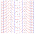 斜率場(黑色)、一些解(紅色)和等斜線(藍色)y'=x
 -
 對應於微分方程dy / dx = x2 − x − 2 的斜率場的三個積分曲線


向量場的視覺化
[edit | edit source]繪圖型別(流資料視覺化技術) : [20]
- 符號 = 用於視覺化向量場的圖示或符號
- 最簡單的符號 = 線段(刺蝟圖)
- 箭頭圖 = 羽毛圖 = 刺蝟(全域性箭頭圖)
- 特徵線 [21]
- 流線 = 在任何地方都與瞬時向量(速度)場相切的曲線(時間無關向量場)。對於時間無關向量場,軌跡線 = 路徑線 = 軌跡線 [22]
- 紋理 (線積分卷積 = LIC)[23]
- 拓撲骨架 [24]
- 不動點提取(雅可比矩陣)
-
 LIC
LIC -
 流線和流管
流線和流管 -
 基於影像的流視覺化
 -
積分曲線
-
 積分曲線
積分曲線
.png)


"path lines, streak lines, and stream lines are identical for stationary flows" Leif Kobbelt[25]
羽毛圖
[edit | edit source]定義
- "羽毛圖顯示速度向量為具有分量 (u,v) 的箭頭,位於點 (x,y)"[26]
流圖
[edit | edit source]- 流圖使用流線
- wolfram:ComplexStreamPlot
fBM 代表分形布朗運動
SDF = 有符號距離函式[27]
- 按維度(1D、2D、3D...)
- 按顏色
- 按距離函式(歐幾里得距離,
- 演算法[28]
- 高效的快速行進方法,
- 射線行進[29]
- 例如行進拋物線,一種線性時間的 CPU 友好演算法。
- 最小腐蝕,一種易於實現的 GPU 友好演算法
- 快速掃描方法
- 更通用的水平集方法。
- 高效的快速行進方法,
- 視覺化(灰色梯度、LSM,
- 簡單的預定義圖形或任意形狀
它不是
- Sqlce 資料庫檔案(.SDF)是由 SQL Server Compact Edition 建立和訪問的資料庫。= SO 中的 sdf 標籤
- SDFormat(模擬描述格式),有時縮寫為 SDF,是一種 XML 格式,用於描述機器人模擬器、視覺化和控制中的物件和環境。
- ScientificDataFormat (SDF) 和 SDF python 包 = 用於讀取、寫入和插值多維資料。Scientific Data Format 是一種基於 HDF5 的開放檔案格式,用於儲存多維資料,例如引數、模擬結果或測量結果。
- SuiteCloud 開發框架(SDF)
- 二維基本圖形的 SDF
- SDF 的法線
- 梯度
- i quilezles : 內部距離(SDF)
- 由 Martin Donald 製作的字形、形狀、字型、有符號距離欄位
- CSC2547 DeepSDF 用於形狀表示的連續有符號距離函式學習
- 由 Ronja 製作的二維有符號距離欄位基礎
- snelly 是由 Jamie Portsmouth 製作的 WebGL SDF 路徑追蹤器
- shadertoy : 由 paniq 製作的 SDF 射線行進四叉樹
- 由 munrocket 製作的 WGSL 二維 SDF 基本圖形
- 透過有符號距離函式定義 3 種形狀
- 維基百科中的有符號距離函式
- 由 I Quilez 製作的二維距離函式
- i quilez : 二維距離梯度函式
- SDF
- 8 點有符號順序歐幾里得距離變換
- 取樣函式的距離變換
- heman
- Chlumsky: msdfgen = 多通道有符號距離欄位生成器
- image-sdf = 命令列工具,它接受一個 4 通道 RGBA 影像並生成一個有符號距離欄位。位掩碼由 alpha 值大於 128 的畫素和任何 RGB 通道值大於 128 的畫素確定。
- fogleman sdf 在 Python 中簡單的 SDF 網格生成
- christopher batty SDFGen 一個簡單的命令列工具,用於從三角形網格生成基於網格的有符號距離欄位(水平集)生成器。
- 磁碟 - 由 iq 製作的二維距離 - 程式碼很好
- 著色器教程 | 由 Suboptimal Engineer 製作的有符號距離欄位入門 程式碼在實際的 shadertoy 中無法執行
- C 程式碼
- WGLS
// The MIT License
// Copyright © 2020 Inigo Quilez
// Permission is hereby granted, free of charge, to any person obtaining a copy of this software and associated documentation files (the "Software"), to deal in the Software without restriction, including without limitation the rights to use, copy, modify, merge, publish, distribute, sublicense, and/or sell copies of the Software, and to permit persons to whom the Software is furnished to do so, subject to the following conditions: The above copyright notice and this permission notice shall be included in all copies or substantial portions of the Software. THE SOFTWARE IS PROVIDED "AS IS", WITHOUT WARRANTY OF ANY KIND, EXPRESS OR IMPLIED, INCLUDING BUT NOT LIMITED TO THE WARRANTIES OF MERCHANTABILITY, FITNESS FOR A PARTICULAR PURPOSE AND NONINFRINGEMENT. IN NO EVENT SHALL THE AUTHORS OR COPYRIGHT HOLDERS BE LIABLE FOR ANY CLAIM, DAMAGES OR OTHER LIABILITY, WHETHER IN AN ACTION OF CONTRACT, TORT OR OTHERWISE, ARISING FROM, OUT OF OR IN CONNECTION WITH THE SOFTWARE OR THE USE OR OTHER DEALINGS IN THE SOFTWARE.
// GSLS

// Signed distance to a disk

// List of some other 2D distances: https://www.shadertoy.com/playlist/MXdSRf
//
// and iquilezles.org/articles/distfunctions2d


float sdCircle( in vec2 p, in float r )
{
    return length(p)-r;
}


void mainImage( out vec4 fragColor, in vec2 fragCoord )
{
	vec2 p = (2.0*fragCoord-iResolution.xy)/iResolution.y;
    vec2 m = (2.0*iMouse.xy-iResolution.xy)/iResolution.y;

	float d = sdCircle(p,0.5);

	// coloring
    vec3 col = (d>0.0) ? vec3(0.9,0.6,0.3) : vec3(0.65,0.85,1.0); // exterior / interior
    col *= 1.0 - exp(-6.0*abs(d)); // adding a black outline ( gray gradient) to the circle
	col *= 0.8 + 0.2*cos(150.0*d); //  adding waves
	col = mix( col, vec3(1.0), 1.0-smoothstep(0.0,0.01,abs(d)) ); // note: adding white border to the circle


	fragColor = vec4(col,1.0);
}
hg_sdf:一個用於構建有符號距離函式的 glsl 庫
- 水星 -
- ink4
- NVScene 2015 會議:如何使用有符號距離函式建立內容(Johann Korndörfer)
- alan zucconi:有符號距離函式
- jcowles - Mercury 的 hg_sdf 庫的 WebGL 友好移植版
- b3dsdf = 一個包含 2D/3D 距離函式、sdf/向量運算和各種實用著色器節點組(159+)的工具包,適用於 Blender 2.83+
-
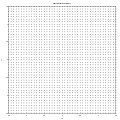 (空)場 : 矩形網格的點
 -
 標量場 : Mandelbrot 集的勢
 -
 向量場:梯度的陣列圖


- 一階、自治的常微分方程組
- 常微分方程組的龍格-庫塔法
- 一階常微分方程組的幾何和數值
- 由 MAKS SURGUY 製作的流線
- symbolab : 常微分方程計算器
- PETSc - 可移植、可擴充套件的科學計算工具包,發音為 PET-see (/ˈpɛt-siː/),用於對由偏微分方程建模的科學應用進行可擴充套件(並行)求解。它具有 C、Fortran 和 Python(透過 petsc4py)的繫結。PETSc 還包含 TAO,即高階最佳化工具包軟體庫。它支援 MPI,以及透過 CUDA、HIP 或 OpenCL 的 GPU,以及混合 MPI-GPU 並行性;它還支援 NEC-SX Tsubasa 向量引擎。
- Maxima CAS
- CGAL - 由 Abdelkrim Mebarki 製作的二維流線放置
- Python
- OpenProcessing
- G'MIC - display_quiver
- OpenCV
- dsp.stackexchange: 如何在影像中檢測梯度 - 方向梯度直方圖 (HOG)
- 箭頭線
- Maxima CAS
- plotdf(用於常微分方程)
- C++
- par_streamlines(C,WebGl) 由 Philip Allan Rideout 製作,github: prideout/par
- JavaScript
- c
- vfplot - 由 J J Green 製作的用於繪製二維向量場的程式
- rk4,由 j burkardt 製作的 C 程式碼,使用四階龍格-庫塔方法求解常微分方程 (ODE)。
- gsl
- js
- 來自 commons 的圖片:Category:Field_lines
- 來自 commons 的圖片:Category:Vector_fields
- fractalforums.org:cruising-through-fractal-flow-fields
- 由 Chris Thomasson 製作
- Deeplearning.ai 的梯度數值逼近
- 粘在尖端:不斷演變的 Julia 集電容器中的電場線,由 Nils Berglund 製作
The coloured curves are the separatrices (i.e. real flow lines reaching infinity) of the complex ODE dz/dt = p(z) = z^4 + O(z^2), where the four roots of p(z) are pictured as the black dots: one fixed at the origin, and the remaining three forming the vertices of an equilateral triangle centered at the origin and rotating.
Bifurcation occurs at certain critical angles of the rotation, where separatrices instantaneously merge to form homoclinic orbits. Following bifurcation, the so-called 'sectorial pairing' is permuted.
There are a total of 5 possible sectorial pairings for the quartic polynomial vector fields (enumerated by the 3rd Catalan number).
Three out of the five possibilities can be seen in 2/3 video, while the remaining two can be seen in part 1/3
In 3/3 example, at a bifurcation we have that either: only two of the four roots are centers (the other two remaining attached to separatrices), or NONE of the roots are centers (a phenomenon which does not occur for the quadratic or cubic polynomial vector fields).
This video is inspired by the work of A. Douady and P. Sentenac. ( rboyce1000)
演算法
- 建立具有所需屬性的多項式
- f(z) = z*g(z) 具有原點的根
- g(z) 是單位根的 3 次根 =

f(z) = z(z^3 - 1)
可以使用 Maxima CAS 進行檢查
 z:x+y*%i;
(%o1)                              %i y + x
(%i2) p:z*(z^3-1);
                                               3
(%o2)                    (%i y + x) ((%i y + x)  - 1)
(%i3) display2d:false;

(%o3) false
(%i4) r:realpart(p);

(%o4) x*((-3*x*y^2)+x^3-1)-y*(3*x^2*y-y^3)
(%i5) m:imagpart(p);

(%o5) x*(3*x^2*y-y^3)+y*((-3*x*y^2)+x^3-1)
(%i6) plotdf([r,m],[x,y]);

(%o6) "/tmp/maxout28945.xmaxima"

(%i8) s:solve([p],[x,y]);

(%o8) [[x = %r1,y = (2*%i*%r1+%i+sqrt(3))/2],
       [x = %r2,y = (2*%i*%r2+%i-sqrt(3))/2],[x = %r3,y = %i*%r3],
       [x = %r4,y = %i*%r4-%i]]
要圍繞原點旋轉它,請將 1 更改為:(不動點的乘子)其中 t 是以轉數為單位的真分數


評論中的原始函式

- ↑ 維基百科中的向量場
- ↑ 維基百科中的歐幾里得向量
- ↑ matlab:梯度函式
- ↑ stackoverflow 問題:是否有任何標準方法可以計算數值梯度
- ↑ 由 Mamy Ratsimbazafy 製作的 nnp_numerical_gradient
- ↑ matrixlab-examples:梯度
- ↑ 由 itectec 製作的 matlab-function-gradient-numerical-gradient
- ↑ numDeriv:grad
- ↑ numpy:梯度
- ↑ 由 Kenneth I. Joy 製作的向量場中粒子追蹤的數值方法
- ↑ 由 David Guichard 和朋友製作的曲線繪製
- ↑ liruics:科學視覺化入門 - 流場
- ↑ what-when-how 的光柵演算法 - 基本計算機圖形學第二部分
- ↑ bolster.academy : 尤拉方法互動式
- ↑ Greg Petrics 的互動式龍格庫塔 4
- ↑ grasshopper3d 論壇:場線 - 如何重建並使其週期性?overrideMobileRedirect=1
- ↑ 三維向量場中臨界點的分類和視覺化。Furuheim 和 Aasen 的碩士論文
- ↑ 三維向量場中臨界點的分類和視覺化。Furuheim 和 Aasen 的碩士論文
- ↑ Weisstein, Eric W. "積分曲線。" 來自 Wolfram 網路資源 MathWorld
- ↑ 來自 TUV 的流動視覺化
- ↑ Tomáš Fabián 的資料視覺化
- ↑ 來自 UCF 的擁擠場景中流動的跡線表示
- ↑ 劉佔平的 lic
- ↑ 流分析和視覺化中的向量場拓撲,作者:陳國寧
- ↑ 向量場視覺化,作者:Leif Kobbelt
- ↑ matlab ref : quiver 圖
- ↑ CedricGuillemet: SDF = 與符號距離場相關的資源(論文、連結、討論、著色器玩具等)的集合
- ↑ 2018 年 Philip Rideout 的距離場
- ↑ ray-march = 透過距離場光線追蹤渲染過程 3D 幾何圖形