如何描述一個迴圈（週期軌道）

週期
週期軌道的穩定性
(迴圈) 置換^[1]
吸引域

週期

這裡的週期是指迭代函式（對映）的週期。^[2]

如果點 z 在 f 下的週期為 p，則

z:\ f^{p}(z)=z

或用另一種表示法

z_{p}=z_{0}

滿足上述條件的最小正整數 p 稱為點 z 的素週期或最小週期。

方程和多項式 F

所以週期點的方程

f^{p}(z)=z

或用另一種表示法

F^{p}(z)=f^{p}(z)-z=0

度數

多項式的度數 d 是多項式中非零係數的單項式（單個項）的度數中最高的值。

有理函式的度數是分子和分母的度數中較高的那個值。

對於迭代的二次多項式

d=deg(f^{p})==2^{p}

如何為給定週期找到週期點？

一種用於計算一些多項式對映的精確 n 迴圈的演算法

視覺檢查

視覺檢查^[3] 臨界軌道有助於

理解動力學
找到週期點

週期為 1，動力學緩慢的軌道
週期為 3 的拋物型軌道
週期為 3 的軌道

符號方法

復二次對映

 f(z,c):=z*z+c;

 fn(p, z, c) :=
  if p=0 then z
  elseif p=1 then f(z,c)
  else f(fn(p-1, z, c),c);

標準多項式Fp，其根是週期為p及其因子的週期z點

數學符號： $\ F_{p}(z,c)=f_{c}^{(p)}(z)-z$ ^[4]
ggplot^[5]
Maxima CAS 函式

F(p, z, c) := fn(p, z, c) - z ;

計算簡化多項式Gp的函式，其根是週期為p的週期z點，但沒有其因子的根

數學定義： $G_{p}(z,c)={\frac {F_{p}(z,c)}{\prod _{m|p,m<p}G_{m}(z,c)}}\,$
Maxima 函式

G[p,z,c]:=
block(
[f:divisors(p),
t:1], /* t is temporary variable = product of Gn for (divisors of p) other than p */
f:delete(p,f), /* delete p from list of divisors */
if p=1
then return(F(p,z,c)),
for i in f do 
 t:t*G[i,z,c],
g: F(p,z,c)/t,
return(ratsimp(g))
)$

查詢週期點的方程式

標準方程式

週期點的方程式對於週期 $p\,$ 是

$\ F_{p}(z,c)=0\,$

因此在 Maxima 中

for i:1 thru 4 step 1 do disp(i,expand(Fn(i,z,c)=0));
1
z^2-z+c=0
2
z^4+2*c*z^2-z+c^2+c=0
3
z^8+4*c*z^6+6*c^2*z^4+2*c*z^4+4*c^3*z^2+4*c^2*z^2-z+c^4+2*c^3+c^2+c=0
4
z^16+8*c*z^14+28*c^2*z^12+4*c*z^12+56*c^3*z^10+24*c^2*z^10+70*c^4*z^8+60*c^3*z^8+6*c^2*z^8+2*c*z^8+56*c^5*z^6+80*c^4*z^6+
24*c^3*z^6+8*c^2*z^6+28*c^6*z^4+60*c^5*z^4+36*c^4*z^4+16*c^3*z^4+4*c^2*z^4+8*c^7*z^2+24*c^6*z^2+24*c^5*z^2+16*c^4*z^2+
8*c^3*z^2- z+c^8+4*c^7+6*c^6+6*c^5+5*c^4+2*c^3+c^2+c=0

標準方程式的次數為 $2^{p}\,$

這些方程式給出了週期為p及其因子的週期點。這是因為這些多項式是較低週期多項式 $G_{p}\,$ 的乘積

for i:1 thru 4 step 1 do disp(i,factor(Fz(i,z,c)));
1
z^2-z+c
2
(z^2-z+c)*(z^2+z+c+1)
3
(z^2-z+c)*(z^6+z^5+3*c*z^4+z^4+2*c*z^3+z^3+3*c^2*z^2+3*c*z^2+z^2+c^2*z+2*c*z+z+c^3+2*c^2+c+1)
4
(z^2-z+c)*(z^2+z+c+1)(z^12+6*c*z^10+z^9+15*c^2*z^8+3*c*z^8+4*c*z^7+20*c^3*z^6+12*c^2*z^6+z^6+6*c^2*z^5+2*c*z^5+15*c^4*z^4+18*c^3*z^4+3*
c^2*z^4+4*c*z^4+4*c^3*z^3+4*c^2*z^3+z^3+6*c^5*z^2+12*c^4*z^2+6*c^3*z^2+5*c^2*z^2+c*z^2+c^4*z+2*c^3*z+c^2*z+2*c*z+c^6+
3*c^5+3*c^4+3*c^3+2*c^2+1)

所以

$\ F_{1}(z,c)=z^{2}-z+c=G_{1}\,$

$\ F_{2}(z,c)=(z^{2}-z+c)*(z^{2}+z+c+1)=G_{1}*G_{2}\,$

$\ F_{3}(z,c)=(z^{2}-z+c)*(z^{6}+z^{5}+3*c*z^{4}+z^{4}+2*c*z^{3}+z^{3}+3*c^{2}*z^{2}+3*c*z^{2}+z^{2}+c^{2}*z+2*c*z+z+c^{3}+2*c^{2}+c+1)=G_{1}*G_{3}\,$

$\ F_{4}(z,c)=G_{1}*G_{2}*G_{4}\,$

$\ F_{5}(z,c)=G_{1}*G_{5}\,$

標準方程可以簡化為方程 $G_{p}\,$ ，給出週期為p的週期點，但不包括其因子。

另請參見：維基百科中的素因子表

簡化方程

簡化方程為

$G_{p}(z,c)=0\,$

所以在 Maxima 中給出

for i:1 thru 5 step 1 do disp(i,expand(G[i,z,c]=0));
1
z^2-z+c=0
2
z^2+z+c+1=0
3
z^6+z^5+3*c*z^4+z^4+2*c*z^3+z^3+3*c^2*z^2+3*c*z^2+z^2+c^2*z+2*c*z+z+c^3+2*c^2+c+1=0
4
z^12+6*c*z^10+z^9+15*c^2*z^8+3*c*z^8+4*c*z^7+20*c^3*z^6+12*c^2*z^6+z^6+6*c^2*z^5+2*c*z^5+15*c^4*z^4+18*c^3*z^4+
3*c^2*z^4+4*c*z^4+4*c^3*z^3+4*c^2*z^3+z^3+6*c^5*z^2+12*c^4*z^2+
6*c^3*z^2+5*c^2*z^2+c*z^2+c^4*z+2*c^3*z+c^2*z+2*c*z+c^6+3*c^5+3*c^4+3*c^3+2*c^2+1=0

週期	degree Fp	degree Gp
1	2^1 = 2	2
2	2^2=4	2
3	2^3 = 8	6
4	2^4 = 16	12
p	d = 2^p

計算週期點

維基百科中的定義 ^[6]

不動點（週期 = 1）

定義不動點的方程

 z^2-z+c = 0

在 Maxima 中

定義 c 值

(%i1) c:%i;
(%o1) %i

計算不動點

(%i2) p:float(rectform(solve([z*z+c=z],[z])));
(%o2) [z=0.62481053384383*%i-0.30024259022012,z=1.30024259022012-0.62481053384383*%i]

找出哪些是排斥的

abs(2*rhs(p[1]));

證明不動點的總和為 1

(%i10) p:solve([z*z+c=z], [z]);
(%o10) [z=-(sqrt(1-4*%i)-1)/2,z=(sqrt(1-4*%i)+1)/2]
(%i14) s:radcan(rhs(p[1]+p[2]));
(%o14) 1

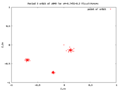
繪製點

(%i15) xx:makelist (realpart(rhs(p[i])), i, 1, length(p));
(%o15) [-0.30024259022012,1.30024259022012]
(%i16) yy:makelist (imagpart(rhs(p[i])), i, 1, length(p));
(%o16) [0.62481053384383,-0.62481053384383]
(%i18) plot2d([discrete,xx,yy], [style, points]);

可以將點 z=1/2 新增到列表中

(%i31) xx:cons(1/2,xx);
(%o31) [1/2,-0.30024259022012,1.30024259022012]
(%i34) yy:cons(0,yy);
(%o34) [0,0.62481053384383,-0.62481053384383]
(%i35) plot2d([discrete,xx,yy], [style, points]);

在 C 中

  
complex double GiveFixed(complex double c){
/* 

Equation defining fixed points : z^2-z+c = 0
	z*2+c = z
	z^2-z+c = 0

coefficients of standard form ax^2+ bx + c  
 	a = 1 , b = -1 , c = c
 
The discriminant d is 

	d=b^2- 4ac 
	d = 1 - 4c
	
 
 alfa =  (1-sqrt(d))/2 
*/

	complex double d = 1-4*c;
	complex double z = (1-csqrt(d))/2.0;
	return z;

}

double complex GiveAlfaFixedPoint(double complex c)
{
  // Equation defining fixed points : z^2-z+c = 0
  // a = 1, b = -1 c = c
  double dx, dy; //The discriminant is the  d=b^2- 4ac = dx+dy*i
  double r; // r(d)=sqrt(dx^2 + dy^2)
  double sx, sy; // s = sqrt(d) = sqrt((r+dx)/2)+-sqrt((r-dx)/2)*i = sx + sy*i
  double ax, ay; // alfa = ax+ay*I
 
 // d=1-4c = dx+dy*i
 dx = 1 - 4*creal(c);
 dy = -4 * cimag(c);
 // r(d)=sqrt(dx^2 + dy^2)
 r = sqrt(dx*dx + dy*dy);
 //sqrt(d) = s =sx +sy*i
 sx = sqrt((r+dx)/2);
 sy = sqrt((r-dx)/2);
 // alfa = ax +ay*i = (1-sqrt(d))/2 = (1-sx + sy*i)/2
 ax = 0.5 - sx/2.0;
 ay =  sy/2.0;

return ax+ay*I;
}

週期為 2 的點

在 Maxima CAS 中使用非簡化方程

(%i2) solve([(z*z+c)^2+c=z], [z]);
(%o2) [z=-(sqrt(-4*c-3)+1)/2,z=(sqrt(-4*c-3)-1)/2,z=-(sqrt(1-4*c)-1)/2,z=(sqrt(1-4*c)+1)/2]

證明 z1+z2 = -1

(%i4) s:radcan(rhs(p[1]+p[2]));
(%o4) -1

證明 z2+z3=1

(%i6) s:radcan(rhs(p[3]+p[4]));
(%o6) 1

簡化方程

  $z^{2}+z+c+1=0$

所以單變數二次多項式的標準係數名稱^[7]

ax^{2}+bx+c

是

 a = 1
 b = 1
 c = c+1

可以使用二次公式^[8] 找到精確解（二次方程的根）：^[9]

 $z_{1,2}={\frac {-b\pm {\sqrt {d}}}{2a}}={\frac {-1\pm {\sqrt {d}}}{2}}$

其中

 $d=b^{2}-4ac=1-4(c+1)=-4c-3$

另一個公式^[10] 可用於求解複數的平方根“

$s={\sqrt {d}}={\sqrt {r}}{\frac {d+r}{|d+r|}}$

其中

r=|d|

所以

週期為 3 的點

在 Maxima CAS 中

kill(all);
remvalue(z);

f(z,c):=z*z+c; /* Complex quadratic map */
 finverseplus(z,c):=sqrt(z-c);
 finverseminus(z,c):=-sqrt(z-c);

/* */
fn(p, z, c) :=
  if p=0 then z
  elseif p=1 then f(z,c)
  else f(fn(p-1, z, c),c);

/*Standard polynomial F_p \, which roots are periodic z-points of period p and its divisors */
F(p, z, c) := fn(p, z, c) - z ;

/* Function for computing reduced polynomial G_p\, which roots are periodic z-points of period p without its divisors*/
G[p,z,c]:=
block(
[f:divisors(p),
t:1], /* t is temporary variable = product of Gn for (divisors of p) other than p */
f:delete(p,f), /* delete p from list of divisors */
if p=1
then return(F(p,z,c)),
for i in f do 
 t:t*G[i,z,c],
g: F(p,z,c)/t,
return(ratsimp(g))
)$

 GiveRoots(g):=
 block(
 [cc:bfallroots(expand(%i*g)=0)],
 cc:map(rhs,cc),/* remove string "c=" */
 cc:map('float,cc),
 return(cc)
  )$

compile(all);

k:G[3,z,c]$
c:1;
s:GiveRoots(ev(k))$
s;

數值方法

wolframalpha

牛頓法

找到一個根

演算法

對於給定的（和固定 = 常數值）

週期 p
引數 c
初始近似值 $z_{0}$ = 牛頓迭代的初始值

尋找一個復二次多項式 $f$ 的週期點 $z$

   $z:f^{p}(z)=z$

其中

   $f(z)=z^{2}+c$

請注意，週期點 $z$ 只是週期迴圈中的 p 個點之一。

為了找到週期點，我們必須解方程（= 找到函式 F 的一個零點）

 $f^{p}(z)-z=0$

我們稱此方程的左側（任意名稱）為函式 $F$

 $F_{p}(z)=f^{p}(z)-z$

函式 $F$ 關於變數 z 的導數

  $F'_{p}(z)=f^{p'}(z)-1$

可以使用 Maxima CAS 檢查

(%i1) f:z*z+c;
(%o1)                                                                                                            z^2  + c
(%i2) F:f-z;
(%o2)                                                                                                          z^2  - z + c
(%i3) diff(F,z,1);
(%o3)                                                                                                           2 z - 1

牛頓迭代是

 $z_{n+1}=z_{n}-{\frac {F_{p}(z_{n})}{F'_{p}(z_{n})}}=z_{n}-{\frac {f_{p}(z_{n})-z_{n}}{f'_{p}(z_{n})-1}}=z_{n}-N_{p}(z_{n})$

給出點 $z_{n}$ 的序列

z_{0}

z_{1}=z_{0}-N_{p}(z_{0})

z_{2}=z_{1}-N_{p}(z_{1})

...

z_{n+1}=z_{n}-N_{p}(z_{n})

其中

n 是牛頓迭代的次數
p 是週期（固定的正整數）
$z_{0}$ 是週期點的初始近似值
$z_{n}$ 是週期點的最終近似值
$f_{p}(z_{n})$ 使用以 $z_{n}$ 為起點的二次迭代計算
$f'_{p}(z_{n})$ 是第一次導數的值。使用迭代計算
$N_{p}$ 稱為牛頓函式。有時使用不同的、更短的符號： $N_{p}(z_{n})=z_{n}-{\frac {F_{p}(z_{n})}{F'_{p}(z_{n})}}$

停止標準

$\epsilon _{succes}$ : 預定義的精度閾值 (succes = 收斂)^[11]
$n_{max}$ : 最大迭代次數 (無法收斂)

$\epsilon =|z_{n+1}-z_{n}|$

通常從

  $\epsilon _{succes}=10^{-16}$

對於長雙精度浮點數格式

  $n_{max}=10^{d}$

精度

精度與多項式 F 的次數成正比，該次數與週期 p 成正比

  $d=d(p)=2^{p-1}$

所以

  $period\to degree\to accuracy\to numberformat$

IEEE 754 - 2008	常用名稱	C++ 資料型別	基數 $b$	精度 $r$	機器精度 = $b^{-(r-1)}$
二進位制16	半精度	short	2	11	2⁻¹⁰ ≈ 9.77e-04
二進位制32	單精度	float	2	24	2⁻²³ ≈ 1.19e-07
二進位制64	雙精度	double	2	53	2⁻⁵² ≈ 2.22e-16
	擴充套件精度	_float80^[12]	2	64	2⁻⁶³ ≈ 1.08e-19
二進位制128	四(重)精度	_float128^[12]	2	113	2⁻¹¹² ≈ 1.93e-34

其中

精度 = 小數部分的二進位制位數
精度 < 機器精度

 precision =  -log2(accuracy)

精度和次數 d 之間的關係:^[13]

精度 = 1/d
精度 = 1/(2 d log d)

比較

使用 Maxima CAS 計算中心點的精度
縮放的精度

迭代次數

程式碼

來自 mandel 的 cpp

c

來自 mandelbrot-numerics 庫的 m-attractor

/* 
gcc -std=c99 -Wall -Wextra -pedantic -O3 m.c -lm
./a.out
*/

#include <complex.h>
#include <math.h>
#include <stdio.h>
#include <stdlib.h>

const double pi = 3.141592653589793;

static inline double cabs2(complex double z) {
  return (creal(z) * creal(z) + cimag(z) * cimag(z));
}

/* 
newton function 
 N(z) = z - (fp(z)-z)/fp'(z)) 
 used for computing periodic point 
 of complex quadratic polynomial
 f(z) = z*z +c

*/

complex double N( complex double c, complex double zn , int pMax, double er2){

  
complex double z = zn;
complex double d = 1.0; /* d = first derivative with respect to z */
int p;

for (p=0; p < pMax; p++){

   
   d = 2*z*d; /* first derivative with respect to z */
   z = z*z +c ; /* complex quadratic polynomial */
   if (cabs(z) >er2) break;
    
}

      z = zn - (z - zn)/(d - 1) ;

return z;
}

/* 
compute periodic point 
of complex quadratic polynomial
using Newton iteration = numerical method

*/

complex double GivePeriodic(complex double c, complex double z0, int period, double eps2, double er2){

complex double z = z0;
complex double zPrev = z0; // prevoiuus value of z
int n ; // iteration
const int nMax = 64;

for (n=0; n<nMax; n++) {
     
    z = N( c, z, period, er2);
    if (cabs2(z - zPrev)< eps2) break;
    
    zPrev = z; }

return z;
}

int main() {

 
 const double ER2  = 2.0 * 2.0; // ER*ER
 const double EPS2 = 1e-100 * 1e-100; // EPS*EPS

  int period = 3;
  complex double c = -0.12565651+0.65720*I ; // https://commons.wikimedia.org/wiki/File:Fatou_componenets_3.png
  complex double z0 = 0.0 ; // initial aproximation for Newton method; usuallly critical point
 
  complex double zp; // periodic point
  
 
  
  
  
  
  zp = GivePeriodic( c , z0, period, EPS2, ER2); //
  
  
  
 
  
  
  printf (" c = %f ; %f \n",  creal(c), cimag(c)); 
  printf (" period = %d  \n",  period); 
  printf (" z0 = %f ; %f \n",  creal(z0), cimag(z0));
  printf (" zp = %.16f ; %.16f \n",  creal(zp), cimag(zp));

  return 0;
}

Maxima CAS

/*

batch file for Maxima CAS

find periodic point of iterated function

solve : 
c0: -0.965 + 0.085*%i$ //     period of critical orbit = 2
2						1 ( alfa ) repelling 						2						1 ( beta) repelling
[0.08997933216560844 %i - 0.972330689471866, 	0.0385332450804691 %i - 0.6029437025417168, 	(- 0.0899793321656081 %i) - 0.02766931052813359, 	1.602943702541716 - 0.03853324508046944 %i] // periodic z points
[1.952970301777068, 				1.208347498712429, 				0.1882750218384916, attr					3.206813573935709] // stability ( 1)
[0.3676955262170045, 				1.460103677644584, 				0.3676955262170032, attr					10.28365329797831] // stability (2)

Newton : 
z0: 0 				 zn : - 0.08997933216560859 %i - 0.02766931052813337
z0: -0.86875-0.03125*%i 	 zn: 0.08997933216560858*%i-0.9723306894718666

(%o21) (-0.08997933216560859*%i)-0.02766931052813337
(%i22) zn2:Periodic(period,c0,(-0.86875)-0.03125*%i,ER,eps)
(%o22) 0.08997933216560858*%i-0.9723306894718666

*/

kill(all); /* if you want to delete all variables and functions. Careful: this does not completely reset the environment to its initial state. */
remvalue(z);
reset(); /*  Resets many (global) system variables */
ratprint : false; /* remove "rat :replaced  " */
display2d:false$ /* display in one line */

mode_declare(ER, real)$
ER: 1e100$
mode_declare(eps,real)$
eps:1e-100$
mode_declare( c0, complex)$
c0: -0.965 + 0.085*%i$ /*     period of critical orbit = 2*/
mode_declare(z0, complex)$
z0:0$
mode_declare(period, integer)$
period:2$

/* ----------- functions  ------------------------ */

/*
 https://wikibook.tw/wiki/Fractals/Iterations_in_the_complex_plane/qpolynomials
complex quadratic polynomial
*/

f(z,c):=z*z+c$

/* iterated map */

fn(p, z, c) :=
  if p=0 then z
  elseif p=1 then f(z,c)
  else f(fn(p-1, z, c),c);
  
  
Fn(p,z,c):=  fn(p, z, c) - z$

  
  
/* find periodic point using solve = symbolic method */  
S(p,c):=
(
s: solve(Fn(p,z,c)=0,z),
s: map( rhs, s),
s: float(rectform(s)))$

/* newton function : N(z) = z - (fp(z)-z)/(f'(z)-1) */

N(zn, c, iMax, _ER):=block(

[z, d], /* d = first derivative with respect to z */
/* mode_declare([z,zn, c,d], complex), */

d  : 1+0*%i,
z  : zn,

catch( for i:1 thru iMax step 1 do (

 
 /*  print("i =",i,", z=",z, ", d = ",d),   */

  
  d : float(rectform(2*z*d)), /* first derivative with respect to z */
  z : float(rectform(z^2+c)), /* complex quadratic polynomial */
  
  
  if ( cabs(z)> _ER)  /* z is escaping */
     then  throw(z)

  )), /* catch(for i */
  
 
   if (d!=0) /* if not : divide by 0 error */ 
     then  z:float(rectform( zn - (z - zn)/(d-1))),
      
   
 return(z) /*  */

)$

/* compute periodic point 
  of complex quadratic polynomial
using Newton iteration = numerical method  */
Periodic(p, c, z0, _ER, _eps) :=block
(
 [z, n, temp], /* local variables */

 if (p<1) 
   then print("to small p ")
   else (

 	n:0,
 	z: z0,  /*  */
 	temp:0,
 	/* print("n = ", n, "zn = ", z ),   */
 
 
        catch(
 	  while (1) do (
 
 		z : N(z, c, p, _ER),   
 		n:n+1,
 		
   	       /*  print("n = ", n, "zn = ", z ),  */
   		
   		
   		if(cabs(temp-z)< _eps) then  throw(z),
   		temp:z,
 
 		if(n>64) then throw(z) ))), /* catch(while) */
 
 	

 
 return(z) 
 
  
  
  )$
  
  
 compile(all)$

/* ------------------ run ---------------------------------------- */

zn1: Periodic(period, c0, z0, ER, eps);   
zn2 : Periodic(period, c0,-0.868750000000000-0.031250000000000*%i, ER, eps);

輸出

(%i21) zn1:Periodic(period,c0,z0,ER,eps)
(%o21) (-0.08997933216560859*%i)-0.02766931052813337
(%i22) zn2:Periodic(period,c0,(-0.86875)-0.03125*%i,ER,eps)
(%o22) 0.08997933216560858*%i-0.9723306894718666

找到所有根

方法

迭代細化牛頓法^[13]
Ehrlich-Aberth 迭代 (Mpsolve^[14])

數量

所有根的數量 = 多項式的次數 (代數基本定理)
次數 = $2^{p}$ 其中 p 是一個週期

週期	度數	所有根的數量
1	2^1 = 2	2
2	2^2=4	4
3	2^3 = 8	8
p	d = 2^p	d

測試

"維埃特公式^[15] 對找到的根進行測試

如果 p 是任何次數為 d 的多項式，並且是歸一化的 (即最高次項係數為 1)，則 p 的所有根的和必須等於 d-1 次項係數的負值。
此外，根的乘積必須等於 (-1)^d 乘以常數項。如果一個根為零，則剩餘 d-1 個根的乘積等於 (-1)^(d-1) 乘以一次項。"

$z_{1}+z_{2}+\dots +z_{d-1}+z_{d}=-{\dfrac {a_{d-1}}{a_{d}}}$

$z_{1}z_{2}\dots z_{d}=(-1)^{d}{\dfrac {a_{0}}{a_{d}}}$

"所有根的總和應為 0 = 多項式的 d − 1 次項的係數 a。"^[16]

$a_{d-1}=0$

$a_{d}=1$

常數項為 a0。它的值取決於週期（次數）。

程式碼

/*

batch file for Maxima CAS

find all periodic point of iterated function
using solve

*/

kill(all);         /* if you want to delete all variables and functions. Careful: this does not completely reset the environment to its initial state. */
remvalue(all);
reset();           /*  Resets many (global) system variables */
ratprint : false;  /* remove "rat :replaced  " */
display2d:false$   /* display in one line */

mode_declare(c0, complex)$
c0: -0.965 + 0.085*%i$ /*     period of critical orbit = 2*/
mode_declare(z, complex)$

mode_declare(period, integer)$
period:2  $

/* ----------- functions  ------------------------ */

/*
 https://wikibook.tw/wiki/Fractals/Iterations_in_the_complex_plane/qpolynomials
complex quadratic polynomial
*/

f(z,c):=z*z+c$

/* iterated map */

fn(p, z, c) :=
  if p=0 then z
  elseif p=1 then f(z,c)
  else f(fn(p-1, z, c),c);
  
  
Fn(p,z,c):=  fn(p, z, c) - z$

  
  
/* find periodic point using solve = symbolic method */  
S(p,c):=
(
s: solve(Fn(p,z,c)=0,z),
s: map( rhs, s),
s: float(rectform(s)))$

/* gives a list of coefficients */
GiveCoefficients(P,x):=block
( [a, degree],
  P:expand(P), /* if not expanded */
  degree:hipow(P,x),
  a:makelist(coeff(P,x,degree-i),i,0,degree));

GiveConstCoefficient(period, z, c):=(
 [l:[]],
 l :  GiveCoefficients( Fn(period,z,c), z),
 l[length(l)]
)$

/*

https://en.wikipedia.org/wiki/Vieta%27s_formulas
sum of all roots , here it should be zero

*/

VietaSum(l):=(
abs(sum(l[i],i, 1, length(l)))

)$

/*

it should be = (-1)^d* a0 = constant coefficient of Fn

*/

VietaProduct(l):=(
rectform(product(l[i],i, 1, length(l)))
)$

compile(all);

s: S(period, c0)$

vs: VietaSum(s);

vp : VietaProduct(s);

a0: GiveConstCoefficient( period, z,c0);

示例結果

週期 p=2 迴圈的方程是

 z^4+2*c*z^2-z+c^2+c = 0

所以 d-1 = 3 係數為 0

$a_{d-1}=a_{3}=0$

$a_{0}=c^{2}+c$

次數 d

 $d=2^{p-1}=2^{2-1}=2^{2}=4$

c= -0.965 + 0.085*i 的四個根是

[0.08997933216560844*%i-0.972330689471866, 0.0385332450804691*%i-0.6029437025417168, (-0.0899793321656081*%i)-0.02766931052813359, 1.602943702541716-0.03853324508046944*%i]

它們的總和是

  $sum=6.938893903907228e-18\approx 0$

它們的乘積是

   $product=(-0.07904999999999943*\%i)-0.04100000000000011\approx a_{0}=c^{2}+c\approx (-0.07905*\%i)-0.04100000000000004$

所以結果通過了韋達定理的檢驗

如何計算週期點的穩定性？

週期點（軌道）的穩定性 - 乘子

乘子（或特徵值，導數) $m(f^{p},z_{0})=\lambda \,$ 是有理對映 $f\,$ 在迴圈點 $z_{0}\,$ 處迭代 $p$ 次時的定義如下

m(f^{p},z_{0})=\lambda ={\begin{cases}f^{p\prime }(z_{0}),&{\mbox{if }}z_{0}\neq \infty \\{\frac {1}{f^{p\prime }(z_{0})}},&{\mbox{if }}z_{0}=\infty \end{cases}}

其中 $f^{p\prime }(z_{0})$ 是 $\ f^{p}$ 關於 $z\,$ 在 $z_{0}$ 處的導數。

因為乘數在給定軌道上的所有周期點都是相同的，所以它被稱為週期軌道的乘數。

乘數是

一個複數；
在任何有理對映在其不動點處的共軛下是不變的；^[17]
用於檢查週期點（也稱為不動點）的穩定性，穩定性指數為 $abs(\lambda ).\,$

一個週期點^[18]

當 $abs(\lambda )<1;\,$ $abs(\lambda )<1;\,$ 時是吸引的；
- 當 $abs(\lambda )=0;\,$ 時是超吸引的；
- 當 $0<abs(\lambda )<1;\,$ 時是吸引的，但不是超吸引的；
當 $abs(\lambda )=1;\,$ $abs(\lambda )=1;\,$ 時是中性的（無差別的）；
- 如果 $\lambda \,$ 是單位根，則它是理性無差別的或拋物線的或弱吸引的^[19]；
- 如果 $abs(\lambda )=1\,$ 但乘數不是單位根，則它是無理性無差別的；
當 $abs(\lambda )>1.\,$ 時是排斥的。

週期點

如果是吸引的，則始終位於法圖集；
如果是排斥的，則位於朱利亞集；
如果是無差別的不動點，則可能位於兩者之一。^[20] 拋物線週期點位於朱利亞集中。

程式碼

c

/* 
gcc -std=c99 -Wall -Wextra -pedantic -O3 m.c -lm

c = -0.965000 ; 0.085000 
 period = 2  
 z0 = 0.000000 ; 0.000000 
 zp = -0.027669 ; -0.089979 
 m = 0.140000 ; 0.340000 
 Internal Angle = 0.187833 
 internal radius = 0.367696 
 
 
 -----------------------------------------
  for (int p = 1; p < pMax; p++){
      
      if( cabs(c)<=2){
      w =  MultiplierMap(c,p);
      iRadius = cabs(w);
      if ( iRadius <= 1.0) { // attractring
           iAngle = GiveTurn(w);
           period=p; 
           break;}
      }   }

*/

#include <complex.h>
#include <math.h>
#include <stdio.h>
#include <stdlib.h>

const double pi = 3.141592653589793;

static inline double cabs2(complex double z) {
  return (creal(z) * creal(z) + cimag(z) * cimag(z));
}

/* newton function : N(z) = z - (fp(z)-z)/f'(z)) */

complex double N( complex double c, complex double zn , int pMax, double er2){

  
complex double z = -zn;
complex double d = -1.0; /* d = first derivative with respect to z */
int p;

for (p=0; p < pMax; p++){

   
   d = 2*z*d; /* first derivative with respect to z */
   z = z*z +c ; /* complex quadratic polynomial */
   if (cabs(z) >er2) break;
    
}

 
 
 
 if ( cabs2(d) > 2) 
     z = zn - (z - zn)/d ;

return z;
}

/* 
compute periodic point 
of complex quadratic polynomial
using Newton iteration = numerical method

*/

complex double GivePeriodic(complex double c, complex double z0, int period, double eps2, double er2){

complex double z = z0;
complex double zPrev = z0; // prevoiuus value of z
int n ; // iteration
const int nMax = 64;

for (n=0; n<nMax; n++) {
     
    z = N( c, z, period, er2);
    if (cabs2(z - zPrev)< eps2) break;
    
    zPrev = z; }

return z;
}

complex double AproximateMultiplierMap(complex double c, int period, double eps2, double er2){
     
     complex double z;  // variable z 
     complex double zp ; // periodic point 
     complex double zcr = 0.0; // critical point
     complex double d = 1;
     
     int p;
     
     // first find periodic point
     zp =  GivePeriodic( c, zcr, period,  eps2, er2); // Find periodic point z0 such that Fp(z0,c)=z0 using Newton's method in one complex variable
     
     // Find w by evaluating first derivative with respect to z of Fp at z0 
     if ( cabs2(zp)<er2) {
     
     
     z = zp;
     for (p=0; p < period; p++){
        d = 2*z*d; /* first derivative with respect to z */
        z = z*z +c ; /* complex quadratic polynomial */
     
     }}
     else d= 10000; //

return d;
}

complex double MultiplierMap(complex double c, int period, double eps2, double er2){

complex double w;
switch(period){
case 1: w = 1.0 - csqrt(1.0-4.0*c); 	break; // explicit
case 2: w = 4.0*c + 4; 			break; //explicit
default:w = AproximateMultiplierMap(c, period, eps2, er2); 	break; //

}

return w;

}

/*
gives argument of complex number in turns 
https://en.wikipedia.org/wiki/Turn_(geometry)

*/

double GiveTurn( double complex z){
double t;

  t =  carg(z);
  t /= 2*pi; // now in turns
  if (t<0.0) t += 1.0; // map from (-1/2,1/2] to [0, 1) 
  return (t);
}

int main() {

  
 const double ER2  = 2.0 * 2.0; // ER*ER
 const double EPS2 = 1e-100 * 1e-100; // EPS*EPS

  int period = 3;
  complex double c = -0.12565651+0.65720*I ; // https://commons.wikimedia.org/wiki/File:Fatou_componenets_3.png
  complex double z0 = 0.0 ; // initial aproximation for Newton method; usuallly critical point
 
  complex double zp; // periodic point
  complex double m; // multiplier
  
 
  
  
  
  
  zp = GivePeriodic( c , z0, period, EPS2, ER2); //
  
  m = MultiplierMap ( c, period,  EPS2, ER2 );
  
 
  
  
  printf (" c = %f ; %f \n",  creal(c), cimag(c)); 
  printf (" period = %d  \n",  period); 
  printf (" z0 = %f ; %f \n",  creal(z0), cimag(z0));
  printf (" zp = %.16f ; %.16f \n",  creal(zp), cimag(zp)); 
  printf (" m = %.16f ; %.16f \n",  creal(m), cimag(m)); 
  printf (" Internal Angle = %.16f \n internal radius = %.16f \n", GiveTurn( m), cabs(m));

  return 0;
}

Maxima CAS

/* 
Computes periodic points 
z: z=f^n(z)
and its stability index ( abs(multiplier(z))

for complex quadratic polynomial :
f(z)=z*z+c

batch file for Maxima cas
Adam Majewski 20090604
fraktal.republika.pl
*/

/* basic function  = monic and centered complex quadratic polynomial 
http://en.wikipedia.org/wiki/Complex_quadratic_polynomial

*/
f(z,c):=z*z+c $

/* iterated function */
fn(n, z, c) :=
    if n=1 	then f(z,c)
			else f(fn(n-1, z, c),c) $
/* roots of Fn are periodic point of  fn function */
Fn(n,z,c):=fn(n, z, c)-z $

/* gives irreducible divisors of polynomial Fn[p,z,c] 
which roots are periodic points of period p */
G[p,z,c]:=
block(
 
 [f:divisors(p),t:1],
 g,
 f:delete(p,f),
 if p=1 
	then return(Fn(p,z,c)),
 for i in f do t:t*G[i,z,c],
 g: Fn(p,z,c)/t,  
 return(ratsimp(g))
  )$
  
  
  
/* use :
load(cpoly); 
roots:GiveRoots_bf(G[3,z,c]);

*/
GiveRoots_bf(g):=
block(
 
 [cc:bfallroots(expand(g)=0)],
 cc:map(rhs,cc),/* remove string "c=" */
 return(cc)
  )$

/* -------------- main ----------------- */
load(cpoly); 
/* c should be inside Mandelbrot set to make attracting periodic points */
/* c:0.74486176661974*%i-0.12256116687665;  center of period 3 component */
coeff:0.37496784+%i*0.21687214; /* -0.11+0.65569999*%i;*/
disp(concat("c=",string(coeff)));

for p:1 step 1 thru 5 do /* period of z-cycle */
( 
 
 disp(concat("period=",string(p))),
/* multiplier */ 
define(m(z),diff(fn(p,z,c),z,1)),

/* G should be found when c is variable without value */
eq:G[p,z,c],  /* here should be c as a symbol not a value */

c:coeff, /* put a value to a symbol here */

/* periodic points */

roots[p]:GiveRoots_bf(ev(eq)), /* ev puts value instead of c symbol */
/* multiplier of periodic points */
for z in roots[p] do disp(concat( "z=",string(float(z)),";     abs(multiplier(z))=",string(cabs(float(m(z)))) ) ),
kill(c)
)$

/*

結果

c:0.74486176661974*%i-0.12256116687665
periodic z-points:
supperattracting cycle (multiplier=0):
3.0879115871966895*10^-15*%i-1.0785250533182843*10^-14=0
0.74486176661974*%i-0.12256116687665=c
0.5622795120623*%i-0.66235897862236=c*c+c

=== repelling cycle
0.038593416246119-1.061217891258986*%i,
0.99358185708018-0.90887310643243*%i,

0.66294971900937*%i-1.247255127827274]
--------------------------------------------

for c:-0.11+0.65569999*%i;
abs(multiplier) = 0.94840556944351

z1a=0.17434140717278*%i-0.23080799291989,
z2a=0.57522120945524*%i-0.087122596659277,
z3a=0.55547045915754*%i-0.4332890929585,

abs(multiplier) =15.06988063154376
z1r=0.0085747730232722-1.05057855305735*%i,
z2r=0.95628667892607-0.89213756745704*%i,
z3r=0.63768304472883*%i-1.213641769411674

如何計算給定週期點的週期？

如何計算真實週期？

Robert Munafo 在 Mu-Ency 中描述的多邊形迭代法
Knighty 的泰勒球迭代法

兩者都可以在一個區域中找到最低週期的核。如果該區域中沒有核（要麼 100% 外部，要麼 100% 內部不圍繞核），我不知道會發生什麼。

多邊形方法可以適應前週期 Misiurewicz 點。泰勒球方法可能也可以。球方法的一個版本可以適應使用雅可比矩陣的燃燒船等，而多邊形方法有時會因早期摺疊而失敗。

int GivePeriod(complex double c){




	if (cabs(c)>2.0) {return 0;} // exterior
	if (cabs(1.0 - csqrt(1.0-4.0*c))<=1.0 ) {return 1;} // main cardioid
	if (cabs(4.0*c + 4)<=1.0){return 2;} // period 2 component
	
	int period =  GivePeriodByIteration(c); 
	
	if ( period < 0) // last chance
		{ 
			iUnknownPeriod +=1;
			//fprintf(stderr,"unknown period = %d < 0 c = %.16f %+.16f \n", period, creal(c), cimag(c) ); // print for analysis
			//period = m_d_box_period_do(c, 0.5, iterMax_LastIteration);
			//fprintf(stderr,"box period = %d  \n", period);
			
		}
	
	// period > 0 means is periodic 
	// period = 0 means is not periodic = exterior = escaping to infinity
	// period < 0 means period not found, maybe increase global variable iterMax_Period ( see local_setup)

	return period; 

}

marcm200

A heuristics to get to a point where the period detection might work correctly could also be: Compute the rolling derivative from the start on, i.e 2^n*product over all iterates. If the orbit approaches an attracting cycle of  length p, cyclic portions of that overall product will become smaller than one in magnitude. And repeatedly multiplying those values will eventually let the |rolling derivative| fall below any ever so small threshold. So if one  were to define beforehand such a small value like 10^-40, if the rolling derivative is first below, then doing a periodicity check by number equaltiy up to an epsilon should give the correct period.  I only use it with unicritical polynomials so chances are that during iteration one does not fall onto a critical point and then the rolling derivative gets stuck at 0 forever (so for z^2+c, starting at c is usually feasible, as +-sqrt(-c) is then almost always irrationally complex and not representable in software. However, with bad luck, its approximation might still lead to computer-0 within machine-epsilon).

( marcm200)

Knighty 的泰勒球迭代法

如 knightly 所建議的那樣，找到 SA 多項式的根是一個完全不同的方法。您使用哪種多項式求根演算法？

ball interval arithmetic" is also called "midpoint-radius interval".

Divide and conquer, using ball interval arithmetic to isolate the roots and Newton-Raphson to refine them.
My approach to Ball interval arithmetic is  very simple:
To a given number z we associate a disc representing an estimation of the errors. A ball interval may be represented like this: [z] = z + r [E]

Here z is the center of the ball, r is the radius and [E] is the error symbol representing the unit disc centred at 0.

Being not a mathematician, be aware that these definitions are very very sloppy. In particular, I don't care about rounding stuff.

One can also think about [E] as a function in some "mute" variables. for example, for complex numbers we can write:
[E] = f(a,b) = a * exp(i *b), where a is in [0,1] and b any real number.
it can also be written like this:
[E]= [0,1] * exp(i * [-inf, +inf])

A nice property of [E] is that raising it to a (positive) power will yield [E].
Another one is: [E] = -[E]
... Another one: z[E] = |z| [E]

Some basic operations on ball interval are:
-Addition:
  [v] + [w] = v + rv [E] + w + rw [E] = (v+w) + (rv+rw) [E]
-Subtraction:
  [v] - [w] = (v-w) + (rv+rw) [E]; because [E] will absorb the '-' sign.
-Multiplication:
 [v] [w] = (v + rv [E]) (w + rw [E]) = v*w + v*rw [E] + w*rv [E] + rv*rw [E]? = v*w + (|v|*rw + |w|*rv + rv*rw) [E]; because [E]? = [E]
The division is more complicated: It is not always defined (when 0 is inside the ball) and needs special care.
-Raising to a power:
use successive multiplications... but that may give too large balls... there are other methods.

With these operations one can evaluate polynomials using Horner method for example. It can also be used to iterate zn+1 = zn? + c for example and be used to find nucleus and its period instead of the box method.

您可以檢視以下程式的程式碼：

檢視此筆記

如何找到吸引點的盆地？

牛頓-拉夫森分形

朱利亞集和週期點之間有什麼關係？

另請參閱

wikibooks 中的 critical_orbit

程式碼

關於使用自相關和函式逼近檢測時間序列資料中的週期和重複模式的一種方法作者：Tim Breitenbach a b，Bartosz Wilkusz b，Lauritz Rasbach b，Patrick Jahnke
- Lauritz R：python 中的週期檢測
- python 週期檢測

參考文獻

[1] Sourav Bhattacharya 和 Alexander Blokh 撰寫的《區間對映的極度無序迴圈》

[2] 維基百科中的週期點

[3] 緩慢動力學下的臨界軌道週期

[4] Scholarpedia 中查詢週期軌道的數值方法

[5] Eric 撰寫的 ggplot2 中的固定點

[6] 維基百科：復二次對映的週期點#有限固定點

[7] 維基百科：二次函式

[8] th.stackexchange 問題：如何找到具有復係數的二次方程的解

[9] 維基百科：二次方程

[10] th.stackexchange 問題：如何求複數的平方根

[11] Dierk Schleicher 和 Robin Stoll 撰寫的《牛頓法在實踐中：有效地查詢一百萬次方多項式的所有根》

[xfloat-12] 浮點型別 - 使用 GNU 編譯器集合 (GCC)

[arxiv.org-13] Robin Stoll 和 Dierk Schleicher 撰寫的《牛頓法在實踐中 II：迭代細化牛頓法和查詢一些非常大次數的多項式的所有根的近乎最優複雜度》

[14] 維基百科：MPSolve

[15] 維基百科：韋達定理

[16] Dierk Schleicher 和 Robin Stoll 撰寫的《牛頓法在實踐中：有效地查詢一百萬次方多項式的所有根》

[17] Alan F. Beardon 撰寫的《有理函式的迭代》，Springer 1991，ISBN 0-387-95151-2，第 41 頁

[18] Alan F. Beardon 撰寫的《有理函式的迭代》，Springer 1991，ISBN 0-387-95151-2，第 99 頁

[19] Monireh Akbari 和 Maryam Rabii 撰寫的《具有雙重固定點的實三次多項式》，《Indagationes Mathematicae》，第 26 卷，第 1 期，2015 年，第 64-74 頁，ISSN 0019-3577，https://doi.org/10.1016/j.indag.2014.06.001. (https://www.sciencedirect.com/science/article/pii/S0019357714000536) 摘要：本文旨在研究具有雙重固定點的實三次多項式的動力學。此類多項式與 fa(x)=ax2(x−1)+x，a≠0 共軛。我們將證明當 a>0 且 x≠1 時，|fan(x)| 收斂於 0 或 ∞，如果 a<0 且 a 屬於引數空間的某個特殊子集，則存在 R 上的一個封閉不變子集 Λa，在該子集上 fa 是混沌的。關鍵詞：重數；混沌；三次多項式；施瓦茨導數

[20] Michael Becker 撰寫的《一些 Julia 集》

[1]

[2]

[3]

[4]

[5]

[6]

[7]

[8]

[9]

[10]

[11]

[12]

[13]

[14]

[15]

[16]

[17]

[18]

[19]

[20]

週期

方程和多項式 F

度數

如何為給定週期找到週期點？

視覺檢查

符號方法

標準多項式Fp，其根是週期為p及其因子的週期z點

計算簡化多項式Gp的函式，其根是週期為p的週期z點，但沒有其因子的根

查詢週期點的方程式

標準方程式

簡化方程

計算週期點

不動點（週期 = 1）

週期為 2 的點

週期為 3 的點

數值方法

牛頓法

找到一個根

演算法

停止標準

精度

迭代次數

程式碼

c

Maxima CAS

找到所有根

測試

程式碼

示例結果

如何計算週期點的穩定性 ？

週期點（軌道）的穩定性 - 乘子

程式碼

c

Maxima CAS

如何計算給定週期點的週期？

marcm200

Knighty 的泰勒球迭代法

如何找到吸引點的盆地？

朱利亞集和週期點之間有什麼關係？

另請參閱

程式碼

參考文獻

如何計算週期點的穩定性？