演算法

[編輯 | 編輯原始碼]

後處理 = 影像修改 = 圖形演算法 = 影像處理

按圖形型別分類的演算法

光柵演算法
向量演算法

五類影像處理演算法

影像恢復
影像分析
影像合成
影像增強
影像壓縮。

列表：^[1]^[2]^[3]

色彩理論：色彩漸變
二維平面變換
- 二維到三維^[4]
  - 高度圖^[5]
  - 坡度

二值影像的形態學運算^[6]^[7]
- 形態學閉運算 = 膨脹後腐蝕
- 形態學開運算 = 腐蝕後膨脹

後處理

兩種邊緣檢測型別
偽三維投影
星空場生成器
隨機點立體圖（又名魔眼）
動畫的運動模糊
隔行掃描
浮雕
反鋸齒
調色盤模擬，允許真彩色顯示器上的顏色迴圈
真彩色模擬，在 256 色顯示器上提供抖動

演算法

使用漸變對映，在分形建立後獨立於分形建立進行著色
- 直方圖著色
密集影像的伽馬校正^[8]
維基百科中的直方圖均衡
（矩陣）卷積（= 離散卷積）是兩個矩陣的逐元素相乘，然後求和
- 影像卷積
  - LIC

型別

[編輯 | 編輯原始碼]

範圍

[編輯 | 編輯原始碼]

影像處理運算子（演算法）可以分為 4 類

畫素演算法 = 畫素處理：點運算子作用於單個畫素：g = H(f)
- 新增兩張影像：g(x)=f1(x)+f2(x)
- 直方圖
- 查詢表（LUT）
- 視窗化
區域性演算法 = 核化 = 區域性處理：“區域性運算子計算畫素值 g(x) 不僅基於輸入影像中相同位置的值，即 f(x)，而且還使用附近點的幾個值 f(x+y)。區域性運算子是幾乎所有影像處理任務的核心。”^[9]
- 空間位置濾波（卷積），
- 使用高通和低通數字濾波器的空間頻率濾波，
- 反銳化遮罩技術^[10]
幾何處理 = 幾何變換：“雖然點運算子改變所有畫素的值，但幾何運算子不改變值，而是將畫素‘移動’到新位置。”
全域性運算子：“全域性運算子（可能）需要輸入影像中的所有畫素值來計算輸出影像中單個畫素的值。”

庫

[編輯 | 編輯原始碼]

數字拓撲

[編輯 | 編輯原始碼]

幾何

[編輯 | 編輯原始碼]

雙曲
- 雙曲

光

[編輯 | 編輯原始碼]

光源

伽馬校正

[編輯 | 編輯原始碼]

gamma 校正 by Mikael Hvidtfeldt Christensen

密集影像

[編輯 | 編輯原始碼]

密集影像^[11]^[12]^[13]^[14]^[15]

帶 gamma 校正的降取樣^[16]
路徑查詢^[17]
混疊 ^[18]
將演算法（表示函式）從離散更改為連續，例如從逃逸時間水平集方法更改為連續（DEM）

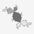
  "the denser the area, the more heavy the anti-aliasing have to be in order to make it look good."  knighty^[19]

  "the details are smaller than pixel spacing, so all that remains is the bands of colour shift from period-doubling of features making it even denser"  claude^[20]

平鋪

[編輯 | 編輯原始碼]

平鋪編輯器
Tiling Bot by Roice Nelson
繪製雙曲平面中均勻平鋪的 Wythoff 構造
EPINET = 非歐幾里得平鋪中的歐幾里得模式

路徑查詢

[編輯 | 編輯原始碼]

路徑查詢

演算法^[21]

深度優先搜尋 (DFS) = 最簡單的演算法
廣度優先搜尋 (BFS)
雙向搜尋
Dijkstra 演算法（或 Dijkstra 最短路徑優先演算法，SPF 演算法）
- programiz：dijkstra-algorithm
- dyclassroom：dijkstra-algorithm-finding-shortest-path
Bellman-Ford 演算法

尺寸

[編輯 | 編輯原始碼]

如何開啟大影像
- vliv: Vliv 背後的原理（只加載可見的影像部分，並利用 TIFF 格式 - 平鋪金字塔影像）可以在任何作業系統上實現。外掛的 API 只有 5 個函式，請參閱 vlivplugins repo 以獲取示例。

調整大小

[編輯 | 編輯原始碼]

方法

Image Magic 調整大小
FF
2^x 影像超解析度
- Final2x
- image-super-resolution

多邊形

[編輯 | 編輯原始碼]

二維多邊形的幾何運算^[22]^[23]

如何判斷一個點位於直線的右側還是左側？

[編輯 | 編輯原始碼]

/* 
  How to tell whether a point is to the right or left side of a line ?

 http://stackoverflow.com/questions/1560492/how-to-tell-whether-a-point-is-to-the-right-or-left-side-of-a-line

  a, b = points
  line = ab
 pont to check = z

  position = sign((Bx - Ax) * (Y - Ay) - (By - Ay) * (X - Ax))
  It is 0 on the line, and +1 on one side, -1 on the other side.

*/

double CheckSide(double Zx, double Zy, double Ax, double Ay, double Bx, double By)
{
  return ((Bx - Ax) * (Zy - Ay) - (By - Ay) * (Zx - Ax));

}

測試點是否在三角形內

[編輯 | 編輯原始碼]

描述^[24]^[25]
javascript 程式碼 ^[26]

/* 
c console program 
gcc t.c -Wall
./a.out

*/

# include <stdio.h>

// 3 points define triangle 
double Zax = -0.250000000000000;
double Zay = 0.433012701892219;
// left when y
double Zlx = -0.112538773749444;  
double Zly = 0.436719687479814 ;

double Zrx = -0.335875821657728;
double Zry = 0.316782798339332;

// points to test 
// = inside triangle 
double Zx = -0.209881783739630;
double Zy =   +0.4;

// outside triangle 
double Zxo = -0.193503885412548  ;
double Zyo = 0.521747636163664;

double Zxo2 = -0.338750000000000;
double Zyo2 = +0.440690927838329;

// ============ http://stackoverflow.com/questions/2049582/how-to-determine-a-point-in-a-2d-triangle
// In general, the simplest (and quite optimal) algorithm is checking on which side of the half-plane created by the edges the point is.
double sign (double  x1, double y1,  double x2, double y2, double x3, double y3)
{
    return (x1 - x3) * (y2 - y3) - (x2 - x3) * (y1 - y3);
}

int  PointInTriangle (double x, double y, double x1, double y1, double x2, double y2, double x3, double y3)
{
    double  b1, b2, b3;

    b1 = sign(x, y, x1, y1, x2, y2) < 0.0;
    b2 = sign(x, y, x2, y2, x3, y3) < 0.0;
    b3 = sign(x, y, x3, y3, x1, y1) < 0.0;

    return ((b1 == b2) && (b2 == b3));
}

int Describe_Position(double Zx, double Zy){
if (PointInTriangle( Zx, Zy, Zax, Zay, Zlx, Zly, Zrx, Zry))
  printf(" Z is inside \n");
  else printf(" Z is outside \n");

return 0;
}

// ======================================

int main(void){

Describe_Position(Zx, Zy);
Describe_Position(Zxo, Zyo);
Describe_Position(Zxo2, Zyo2);

return 0;
}

三角形的朝向和麵積

[編輯 | 編輯原始碼]

三角形的朝向和麵積：如何操作？

// gcc t.c -Wall
// ./a.out
# include <stdio.h>

// http://ncalculators.com/geometry/triangle-area-by-3-points.htm
double GiveTriangleArea(double xa, double ya, double xb, double yb, double xc, double yc)
{
return ((xb*ya-xa*yb)+(xc*yb-xb*yc)+(xa*yc-xc*ya))/2.0;
}

/*

wiki Curve_orientation
[http://mathoverflow.net/questions/44096/detecting-whether-directed-cycle-is-clockwise-or-counterclockwise]

The orientation of a triangle (clockwise/counterclockwise) is the sign of the determinant

matrix = { {1 , x1, y1}, {1 ,x2, y2} , {1,  x3, y3}}

where 
(x_1,y_1), (x_2,y_2), (x_3,y_3)$ 
are the Cartesian coordinates of the three vertices of the triangle.

:<math>\mathbf{O} = \begin{bmatrix}

1 & x_{A} & y_{A} \\
1 & x_{B} & y_{B} \\
1 & x_{C} & y_{C}\end{bmatrix}.</math>

A formula for its determinant may be obtained, e.g., using the method of [[cofactor expansion]]:
:<math>\begin{align}
\det(O) &= 1\begin{vmatrix}x_{B}&y_{B}\\x_{C}&y_{C}\end{vmatrix}
-x_{A}\begin{vmatrix}1&y_{B}\\1&y_{C}\end{vmatrix}
+y_{A}\begin{vmatrix}1&x_{B}\\1&x_{C}\end{vmatrix} \\
&= x_{B}y_{C}-y_{B}x_{C}-x_{A}y_{C}+x_{A}y_{B}+y_{A}x_{C}-y_{A}x_{B} \\
&= (x_{B}y_{C}+x_{A}y_{B}+y_{A}x_{C})-(y_{A}x_{B}+y_{B}x_{C}+x_{A}y_{C}).
\end{align}
</math>

If the determinant is negative, then the polygon is oriented clockwise.  If the determinant is positive, the polygon is oriented counterclockwise.  The determinant  is non-zero if points A, B, and C are non-[[collinear]].  In the above example, with points ordered A, B, C, etc., the determinant is negative, and therefore the polygon is clockwise.

*/

double IsTriangleCounterclockwise(double xa, double ya, double xb, double yb, double xc, double yc)
{return  ((xb*yc + xa*yb +ya*xc) - (ya*xb +yb*xc + xa*yc)); }

int DescribeTriangle(double xa, double ya, double xb, double yb, double xc, double yc)
{
 double t = IsTriangleCounterclockwise( xa,  ya, xb,  yb,  xc,  yc);
 double a = GiveTriangleArea( xa,  ya, xb,  yb,  xc,  yc);
 if (t>0)  printf("this triangle is oriented counterclockwise,     determinent = %f ; area = %f\n", t,a);
 if (t<0)  printf("this triangle is oriented clockwise,            determinent = %f; area = %f\n", t,a);
 if (t==0) printf("this triangle is degenerate: colinear or identical points, determinent = %f; area = %f\n", t,a);

 return 0;
}

int main()
{
 // clockwise oriented triangles 
 DescribeTriangle(-94,   0,  92,  68, 400, 180); // https://www-sop.inria.fr/prisme/fiches/Arithmetique/index.html.en
 DescribeTriangle(4.0, 1.0, 0.0, 9.0, 8.0, 3.0); // clockwise orientation https://people.sc.fsu.edu/~jburkardt/datasets/triangles/tex5.txt
 
 //  counterclockwise oriented triangles
 DescribeTriangle(-50.00, 0.00, 50.00,  0.00, 0.00,  0.02); // a "cap" triangle. This example has an area of 1.
 DescribeTriangle(0.0,  0.0, 3.0,  0.0, 0.0,  4.0); // a right triangle. This example has an area of (?? 3 ??)  =  6
 DescribeTriangle(4.0, 1.0, 8.0, 3.0, 0.0, 9.0);  //      https://people.sc.fsu.edu/~jburkardt/datasets/triangles/tex1.txt
 DescribeTriangle(-0.5, 0.0,  0.5,  0.0, 0.0,  0.866025403784439); // an equilateral triangle. This triangle has an area of sqrt(3)/4.

 // degenerate triangles 
 DescribeTriangle(1.0, 0.0, 2.0, 2.0, 3.0, 4.0); // This triangle is degenerate: 3 colinear points. https://people.sc.fsu.edu/~jburkardt/datasets/triangles/tex6.txt
 DescribeTriangle(4.0, 1.0, 0.0, 9.0, 4.0, 1.0); //2 identical points 
 DescribeTriangle(2.0, 3.0, 2.0, 3.0, 2.0, 3.0); // 3 identical points

 return 0; 
}

測試點是否在多邊形內

[編輯 | 編輯原始碼]

stackoverflow^[27]
由 W Muła 描述^[28]
point_in_polygon by Patrick Glauner
- 複雜多邊形的點在多邊形問題中一個簡單且正確的奇偶演算法 by Michael Galetzka, Patrick O. Glauner
- c 程式碼
PNPOLY - 點在多邊形內測試 - W. Randolph Franklin (WRF)

/*

gcc p.c -Wall
./a.out

----------- git --------------------
cd existing_folder
git init
git remote add origin git@gitlab.com:adammajewski/PointInPolygonTest_c.git
git add .
git commit
git push -u origin master

*/

#include <stdio.h>

#define LENGTH 6

/*

Argument	Meaning
nvert	Number of vertices in the polygon. Whether to repeat the first vertex at the end is discussed below.
vertx, verty	Arrays containing the x- and y-coordinates of the polygon's vertices.
testx, testy	X- and y-coordinate of the test point.

https://www.ecse.rpi.edu/Homepages/wrf/Research/Short_Notes/pnpoly.html
PNPOLY - Point Inclusion in Polygon Test
W. Randolph Franklin (WRF)

	

I run a semi-infinite ray horizontally (increasing x, fixed y) out from the test point, 
and count how many edges it crosses. 
At each crossing, the ray switches between inside and outside. 
This is called the Jordan curve theorem.
The case of the ray going thru a vertex is handled correctly via a careful selection of inequalities. 
Don't mess with this code unless you're familiar with the idea of Simulation of Simplicity. 
This pretends to shift the ray infinitesimally down so that it either clearly intersects, or clearly doesn't touch. 
Since this is merely a conceptual, infinitesimal, shift, it never creates an intersection that didn't exist before, 
and never destroys an intersection that clearly existed before.

The ray is tested against each edge thus:

Is the point in the half-plane to the left of the extended edge? and
Is the point's Y coordinate within the edge's Y-range?
Handling endpoints here is tricky.

I run a semi-infinite ray horizontally (increasing x, fixed y) out from the test point, 
and count how many edges it crosses. At each crossing, 
the ray switches between inside and outside. This is called the Jordan curve theorem.
The variable c is switching from 0 to 1 and 1 to 0 each time the horizontal ray crosses any edge. 
So basically it's keeping track of whether the number of edges crossed are even or odd. 
0 means even and 1 means odd.

*/

int pnpoly(int nvert, double *vertx, double *verty, double testx, double testy)
{
  int i, j, c = 0;
  for (i = 0, j = nvert-1; i < nvert; j = i++) {
    if ( ((verty[i]>testy) != (verty[j]>testy)) &&
	 (testx < (vertx[j]-vertx[i]) * (testy-verty[i]) / (verty[j]-verty[i]) + vertx[i]) )
       c = !c;
  }

  return c;
}

void CheckPoint(int nvert, double *vertx, double *verty, double testx, double testy){

int flag;

flag =  pnpoly(nvert, vertx, verty, testx, testy);

 switch(flag){
   case 0  : printf("outside\n"); break;
   case 1  : printf("inside\n"); break;
   default : printf(" ??? \n");
 }
}

int main (){

// values from http://stackoverflow.com/questions/217578/how-can-i-determine-whether-a-2d-point-is-within-a-polygon
// number from 0 to (LENGTH-1)
double zzx[LENGTH] = { 13.5,  6.0, 13.5, 42.5, 39.5, 42.5};
double zzy[LENGTH] = {100.0, 70.5, 41.5, 56.5, 69.5, 84.5};

CheckPoint(LENGTH, zzx, zzy, zzx[4]-0.001, zzy[4]);
CheckPoint(LENGTH, zzx, zzy, zzx[4]+0.001, zzy[4]);

return 0;
}

曲線

[編輯 | 編輯原始碼]

型別

閉合/開放
帶/不帶多個點

方法

追蹤/繪製：生成離散曲線
草繪
取樣
路徑查詢或尋路是指計算機應用程式繪製兩個點之間最短路線的過程
裁剪
數字化曲線的逼近（使用三次貝塞爾曲線）
曲線擬合^[29]
修復斷線^[30]
邊緣檢測

示例

直線
- bresenhams-drawing-algorithms^[31]^[32]^[33]^[34]
- 反鋸齒^[35]

圓形 ^[36]

莫頓碼

[編輯 | 編輯原始碼]

libmorton 帶有方法的 C++ 純標頭檔案庫，可有效地在 2D/3D 座標中對莫頓碼進行編碼/解碼
aavenel mortonlib

變形

[編輯 | 編輯原始碼]

p5.js 中從圓形到三角形的插值 by Golan Levin

曲線簡化

[編輯 | 編輯原始碼]

減少點數，但仍保持曲線的整體形狀 = 折線縮減

曲線擬合

[編輯 | 編輯原始碼]

我的曲線擬合：線上曲線擬合

粗線繪製

[編輯 | 編輯原始碼]

粗線

曲線繪製

[編輯 | 編輯原始碼]

用於光柵顯示的曲線繪製演算法，作者：JERRY VAN AKEN 和 MARK NOVAK
用於繪製曲線的柵格化演算法，作者：Alois Zingl Wien，2012 年
用於光柵顯示的曲線繪製演算法，作者：JERRY VAN AKEN 和 MARK NOVAK
A* 路徑查詢入門，作者：Patrick Lester（更新於 2005 年 7 月 18 日）
Max K. Agoston 計算機圖形學與幾何建模：實現與演算法
libspiro 是 Raph Levien 的作品。它簡化了繪製美麗曲線的過程。
spiro 基於螺旋線的插值樣條曲線

2D 演算法的鄰域變體

8 向步進 (8WS) 用於畫素 p(x, y) 的 8 個方向鄰居
4 向步進 (4WS) 用於畫素 p(x, y) 的 4 個方向鄰居

2D 鄰域
4
8

曲線取樣

[編輯 | 編輯原始碼]

均勻 = 給出等距點
自適應。“一種自適應方法，用於根據局部曲率對域進行取樣。取樣集中度與該曲率成正比，從而產生更有效的近似——極限情況下，一條平坦曲線僅用兩個端點來近似。” ^[38]

場線

[編輯 | 編輯原始碼]

場線^[39]

追蹤

[編輯 | 編輯原始碼]

追蹤曲線^[40]

方法

一般，（解析或系統化） = 曲線繪製^[41]
區域性方法

任務：繪製 2D 曲線，當

沒有直線方程
直線在一定範圍內所有數值

追蹤角度為 t（以圈為單位）的外射線，這意味著（Claude Heiland-Allen 描述）^[42]

從一個大圓圈開始（例如，r = 65536，x = r cos(2 pi t)，y = r sin(2 pi t)）
沿著逃逸線（如使用大逃逸半徑的二進位制分解著色邊的邊緣）向曼德勃羅集內部移動。

此演算法為 O(period^2)，這意味著週期加倍需要 4 倍的時間，因此它僅適用於週期不超過幾千的演算法。

三種曲線追蹤模型^[43]

逐畫素追蹤
暴力法^[44]: 如果您的直線足夠短（小於 10^6 個點），您可以透過計算點 p 到離散直線上每個點的距離來實現，並取這些距離的最小值。
二分感受野運算元
變焦鏡頭運算元

影像

commons 中曲線追蹤類別下的影像

問題

交集和廣度優先搜尋^[45]

示例

向量場中粒子追蹤的數值方法，作者：Kenneth I. Joy

曲線柵格化

[編輯 | 編輯原始碼]

射線

[編輯 | 編輯原始碼]

射線可以使用半徑 (r) 進行引數化

閉合曲線

[編輯 | 編輯原始碼]

簡單閉合曲線（“一條連線的曲線，它不與自身相交，並且在開始點結束”^[46] = 沒有端點）可以使用角度 (t) 進行引數化。

邊界、輪廓、邊緣

[編輯 | 編輯原始碼]

填充輪廓
在二進位制影像中查詢輪廓
CavalierContoursWebDemo 以及程式碼

輪廓模型

[編輯 | 編輯原始碼]

蛇形線 = 活動輪廓模型^[47]

邊界追蹤

[編輯 | 編輯原始碼]

輪廓追蹤演算法，作者：Abeer George Ghuneim
二維影像中的邊界追蹤，作者：V. Kovalevsky^[48]
維基百科 : 邊界追蹤
計算二維標量場的輪廓曲線
- 用於追蹤標量二維場上的輪廓曲線的遊走方塊演算法^[49]
平滑輪廓^[50]
輪廓多邊形^[51]
boundary in C++ by Shawn Halayka - 2019 and new code
opencv_contour in C++ by Shawn Halayka
CONREC，由 Paul Bourke 於 1987 年 7 月編寫的輪廓子例程（使用三角測量）

填充輪廓

[編輯 | 編輯原始碼]

填充輪廓 - c語言中的簡單過程

邊緣檢測

[編輯 | 編輯原始碼]

等高線 - 邊緣檢測（2 個濾波器）
逃逸時間等值面的邊界邊緣檢測

Sobel 濾波器

[編輯 | 編輯原始碼]

簡要介紹

[編輯 | 編輯原始碼]

Sobel 濾波器 G 由 2 個核（掩碼）組成

Gh 用於水平變化。
Gv 用於垂直變化。

Sobel 核

[編輯 | 編輯原始碼]

Sobel 核包含來自測試畫素的 8 點鄰域中每個畫素的權重。這些是 3x3 核。

有兩個 Sobel 核，一個用於計算水平變化，另一個用於計算垂直變化。請注意，大的水平變化可能表明垂直邊界，而大的垂直變化可能表明水平邊界。這裡的 x 座標定義為在“向右”方向上增加，y 座標定義為在“向下”方向上增加。

用於計算水平變化的 Sobel 核為

\mathbf {H} ={\begin{bmatrix}H_{1}&H_{2}&H_{3}\\H_{4}&H_{5}&H_{6}\\H_{7}&H_{8}&H_{9}\end{bmatrix}}={\begin{bmatrix}-1&0&+1\\-2&0&+2\\-1&0&+1\end{bmatrix}}

用於計算垂直變化的 Sobel 核為

\mathbf {V} ={\begin{bmatrix}-1&-2&-1\\\ \ 0&\ \ 0&\ \ 0\\+1&+2&+1\end{bmatrix}}

請注意

核心的權重總和為零

$\sum _{i=1}^{9}H_{i}=0$

$\sum _{i=1}^{9}V_{i}=0$

一個核心只是另一個核心旋轉 90 度。^[53]
每個核心中的 3 個權重為零。

畫素核心

[編輯 | 編輯原始碼]

包含中心畫素 $A_{5}$ 及其 3x3 鄰域的畫素核心 A

\mathbf {A} ={\begin{bmatrix}A_{1}&A_{2}&A_{3}\\A_{4}&A_{5}&A_{6}\\A_{7}&A_{8}&A_{9}\end{bmatrix}}

畫素核心的其他符號

\mathbf {A} ={\begin{bmatrix}A_{1}&A_{2}&A_{3}\\A_{4}&A_{5}&A_{6}\\A_{7}&A_{8}&A_{9}\end{bmatrix}}={\begin{bmatrix}ul&um&ur\\ml&mm&mr\\ll&lm&lr\end{bmatrix}}

其中：^[54]

unsigned char ul, // upper left
unsigned char um, // upper middle
unsigned char ur, // upper right
unsigned char ml, // middle left
unsigned char mm, // middle = central pixel
unsigned char mr, // middle right
unsigned char ll, // lower left
unsigned char lm, // lower middle
unsigned char lr, // lower right

在陣列表示法中，它是：^[55]

\mathbf {A} ={\begin{bmatrix}A[x-1][y+1]&A[x][y+1]&A[x+1][y+1]\\A[x-1][y]&A[x][y]&A[x+1][y]\\A[x-1][y-1]&A[x][y-1]&A[x+1][y-1]\end{bmatrix}}

在細胞自動機中使用的地理表示法中，它是 Moore 鄰域的中心畫素。^{[check spelling]}

因此，中心（測試）畫素是

$A_{5}=mm=A[x][y]\,$

Sobel 濾波器

[edit | edit source]

計算 Sobel 濾波器（其中 $*$ 表示二維卷積運算，而不是矩陣乘法）。它是畫素及其權重的乘積之和

\mathbf {G} _{h}=\mathbf {H} *A=A_{1}H_{1}+A_{2}H_{2}+\cdots +A_{9}H_{9}=\sum _{r=1}^{9}A_{r}H_{r},

\mathbf {G} _{v}=\mathbf {V} *A=A_{1}V_{1}+A_{2}V_{2}+\cdots +A_{9}V_{9}=\sum _{r=1}^{9}A_{r}V_{r},

因為每個核心中的 3 個權重為零，所以只有 6 個乘積。^[56]

short Gh = ur + 2*mr + lr - ul - 2*ml - ll;
short Gv = ul + 2*um + ur - ll - 2*lm - lr;

結果

[edit | edit source]

計算結果（梯度大小）

\mathbf {G} (A_{5})={\sqrt {{\mathbf {G} _{h}}^{2}+{\mathbf {G} _{v}}^{2}}}

它是測試畫素的顏色。

還可以透過兩個幅度之和來近似結果

\mathbf {G} (A_{5})=\left|\mathbf {G} _{h}\right|+\left|\mathbf {G} _{v}\right|

這比計算快得多。^[57]

演算法

[edit | edit source]

選擇畫素及其 3x3 鄰域 A
計算水平 Gh 和垂直 Gv 的 Sobel 濾波器
計算 Sobel 濾波器 G
計算畫素的顏色

程式設計

[edit | edit source]

我們來取一個稱為 data 的 8 位顏色陣列 (影像)。要在這個影像中找到邊界，只需執行以下操作

for(iY=1;iY<iYmax-1;++iY){ 
    for(iX=1;iX<iXmax-1;++iX){ 
     Gv= - data[iY-1][iX-1] - 2*data[iY-1][iX] - data[iY-1][iX+1] + data[iY+1][iX-1] + 2*data[iY+1][iX] + data[iY+1][iX+1];
     Gh= - data[iY+1][iX-1] + data[iY-1][iX+1] - 2*data[iY][iX-1] + 2*data[iY][iX+1] - data[iY-1][iX-1] + data[iY+1][iX+1];
     G = sqrt(Gh*Gh + Gv*Gv);
     if (G==0) {edge[iY][iX]=255;} /* background */
         else {edge[iY][iX]=0;}  /* boundary */
    }
  }

注意，這裡跳過了陣列邊界上的點 (iY= 0, iY = iYmax, iX=0, iX=iXmax)

結果儲存到另一個稱為 edge 的陣列 (大小相同) 中。

可以將 edge 陣列儲存到檔案中，只顯示邊界，或者合併 2 個數組

for(iY=1;iY<iYmax-1;++iY){ 
    for(iX=1;iX<iXmax-1;++iX){ if (edge[iY][iX]==0) data[iY][iX]=0;}}

以生成一個新的帶有標記邊界的影像。

上面的示例適用於 8 位或索引顏色。對於更高位的顏色，“公式分別應用於所有三個顏色通道”(來自 RoboRealm 文件)。

其他實現

問題

[edit | edit source]

在影像中間看到糟糕的邊緣位置。線條沒有在好的點相遇，例如 z = 0

邊緣位置:

在 ImageMagick 中，正如“您所看到的，邊緣只新增到顏色梯度大於 50% 白色的區域！我不知道這是錯誤還是有意為之，但這意味著上面邊緣的位置幾乎完全位於原始掩碼影像的白色部分。這個事實對於使用“-edge”運算子的結果非常重要。”^[58]

結果是

邊緣加倍；“如果你要對包含黑色輪廓的影像進行邊緣檢測，“-edge”運算子會‘雙重’黑色線條，產生奇怪的結果。”^[59]
線條沒有在好的點相遇。

另請參閱 ImageMagick 第 6 版中的新運算子：EdgeIn 和 EdgeOut，來自形態學^[60]

邊緣加厚

[edit | edit source]

膨脹^[61]^[62]^[63]

convert $tmp0 -convolve "1,1,1,1,1,1,1,1,1" -threshold 0 $outfile

SDF 簽名距離函式

[edit | edit source]

向量場 SDF

測試 2 個圓的外切

[edit | edit source]

/*
 distance between 2 points 
  z1 = x1 + y1*I
  z2 = x2 + y2*I
  en.wikipedia.org/wiki/Distance#Geometry
 
*/ 
 
double GiveDistance(int x1, int y1, int x2, int y2){
  return sqrt((x1-x2)*(x1-x2) + (y1-y2)*(y1-y2));
}

/*
mutually and externally tangent circles
mathworld.wolfram.com/TangentCircles.html
Two circles are mutually and externally tangent if distance between their centers is equal to the sum of their radii

*/

double TestTangency(int x1, int y1, int r1, int x2, int y2, int r2){
  double distance;

  distance = GiveDistance(x1, y1, x2, y2);
  return ( distance - (r1+r2));
// return should be zero
}

地圖投影

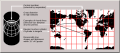
[edit | edit source]

立體投影

[edit | edit source]

立體投影是從球體的北極 N 到球體南極 S 的切平面上點 P' 上的球體表面上點 P 的投影得到的對映投影。^[64]

將北極 N 設為標準單位向量 (0, 0, 1)，並將球體中心設為原點，這樣南極處的切平面就有方程 z = 1。給定單位球體上的一個點 P = (x, y, z)，該點不是北極，它的像等於^[65]

 $P'=f(P)=({\frac {2x}{1-z}},{\frac {2y}{1-z}})=(u,v)$

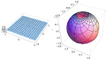平面上的笛卡爾網格在球體上看起來是扭曲的。網格線仍然垂直，但網格正方形的面積隨著它們接近北極而減小。
平面上的極座標網格在球體上看起來是扭曲的。網格曲線仍然垂直，但網格扇區的面積隨著它們接近北極而減小

圓柱形

[edit | edit source]

Cylindrical projections in general have an increased vertical stretching as one moves towards either of the poles. Indeed, the poles themselves can't be represented (except at infinity). This stretching is reduced in the  Mercator projection by the natural logarithm scaling. ^[66]

墨卡託投影

[edit | edit source]

共形
圓柱形 = 墨卡託投影從球體對映到圓柱體。圓柱體沿 y 軸切割並展開。它在兩個 y 方向上都給出了無限範圍的矩形（參見截斷）

圓柱形
標準墨卡託 (圓柱形)
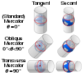墨卡託投影比較

標準墨卡託投影的兩種等效構造

從球體到圓柱體 (一步)
2 步
- 使用標準立體投影將球體投影到一箇中間 (立體) 平面，該投影是共形的
- 透過將立體平面等同於複平面 (該平面在複對數函式下的像，該函式除了原點（帶有一個分支割線）以外都是共形的，

複對數 f(z) = ln(z)。實際上，極座標為 (ρ,θ) 的複數 z 被對映到 f(z) = ln(ρ) + iθ。這會產生一個水平條帶，

然後旋轉 90° 後得到標準垂直墨卡託對映，或者等效地，f(z) 可以定義為 f(z) = i*ln(z)。

	正墨卡託		橫墨卡託
		\

拉伸

[edit | edit source]

Cylindrical projections in general have an increased vertical stretching as one moves towards either of the poles. Indeed, the poles themselves can't be represented (except at infinity). This stretching is reduced in the  Mercator projection by the natural logarithm scaling. ^[67]

截斷

[edit | edit source]

圓柱體不是無限的，因此墨卡託投影在球體兩極產生越來越扭曲的無限條帶。因此，墨卡託投影的座標 y 在兩極處變為無窮大，並且地圖必須在小於 90 度的某個緯度處被截斷（裁剪）。

這不必對稱地進行

墨卡託的原始地圖被截斷在北緯 80° 和南緯 66°，結果是歐洲國家被移到了地圖的中心。

地球的幾何形狀

[edit | edit source]

地球作為球體

地球地理座標系 $(\phi ,\lambda )$

緯度是指地球或其他天體表面上一點的南北位置的座標。緯度通常用角度表示，範圍從南極的 –90° 到北極的 90°，赤道為 0°。緯度通常用希臘字母 phi ( $ϕ$ 或 $φ$ ) 表示。緯度以度、分、秒或十進位制度為單位，以赤道為基準，分別向南北方向測量。
經度是指地球表面上一點的東-西位置的地理座標。經度通常用角度測量，通常以度為單位，用希臘字母 lambda (λ) 表示。

從球體模型上看，地球顯示了緯度 ( $\phi$ ) 和經度 ( $\lambda$ ) 的定義。網格間距為 10 度。

方程

[編輯 | 編輯原始碼]

一步法

考慮一個半徑為 R、經度為 λ、緯度為 φ 的地球上的點。λ₀ 的值為任意中心子午線的經度，通常但並非總是格林尼治子午線（即零度經線）。角度 λ 和 φ 以弧度表示。

將單位球面上的點 P $P=(R,\lambda ,\varphi )$ 對映到笛卡爾平面上的點 $Q=(x,y)$

{\begin{matrix}x=R(\lambda -\lambda _{0})\\y=R\ln \left[\tan \left({\frac {\pi }{4}}+{\frac {\varphi }{2}}\right)\right]\end{matrix}}

兩步法

立體投影
複對數

立體投影的球面形式通常用極座標表示

{\begin{matrix}r&=2R\tan \left({\frac {\pi }{4}}-{\frac {\varphi }{2}}\right)\\\theta &=\lambda \end{matrix}}

其中 $R$ 是球體的半徑， $\varphi$ 和 $\lambda$ 分別是緯度和經度。

直角座標

假設：A、B、C 和 D 是實數，使得 $A^{2}+B^{2}+C^{2}\neq 0$ .

定義

$\Sigma$ 定義為歐幾里德空間中的單位球面，即

   $\Sigma :={\big \{}(x,y,z)\in \mathbb {R} ^{3}:x^{2}+y^{2}+z^{2}=1{\big \}}.$

$N$ 定義為單位球體的北極，即 $N:=(0,0,1)$ .
$S$ 定義為立體投影，即函式 $S:\Sigma \setminus \{N\}\rightarrow \mathbb {R} ^{2}$ 滿足

   $Q=S{\big (}(x,y,z){\big )}={\Big (}{\frac {x}{1-z}},{\frac {y}{1-z}}{\Big )}$

對於每一個 $(x,y,z)\in \Sigma \setminus \{N\}$ .

圓柱座標

圓柱座標 (軸向半徑 ρ, 方位角 φ, 高度 z) 可以透過以下公式轉換為球座標 (中心半徑 r, 傾角 θ, 方位角 φ)

${\begin{aligned}r&={\sqrt {\rho ^{2}+z^{2}}},\\\theta &=\arctan {\frac {\rho }{z}}=\arccos {\frac {z}{\sqrt {\rho ^{2}+z^{2}}}},\\\varphi &=\varphi .\end{aligned}}$

反之，球座標可以透過以下公式轉換為圓柱座標

${\begin{aligned}\rho &=r\sin \theta ,\\\varphi &=\varphi ,\\z&=r\cos \theta .\end{aligned}}$

這些公式假設兩個系統具有相同的原點和相同的參考平面，以相同的方式從相同的軸測量方位角 $φ$ ，並且球面角 $θ$ 是從圓柱形 $z$ 軸的傾角。

程式碼

chinhsuanwu: 360-converter (一個 C/C++ 的 360 影像轉換工具包)

訊號處理

[edit | edit source]

線性連續時間濾波器

頻率響應可以被分為多個不同的帶形，描述了濾波器允許透過的頻率頻段（通帶）和濾波器拒絕的頻率（阻帶）
- 低通濾波器 – 透過低頻，衰減高頻。
- 高通濾波器 – 透過高頻，衰減低頻。
- 帶通濾波器 – 只允許透過某個頻率範圍內的頻率。
- 帶阻濾波器或帶陷濾波器 – 只衰減某個頻率範圍內的頻率。
- 陷波濾波器 – 只拒絕一個特定頻率 - 一種極端的帶阻濾波器。
- 梳狀濾波器 – 具有多個規則間隔的窄通帶，使帶形呈現梳狀外觀。
- 全通濾波器 – 所有頻率都透過，但輸出的相位會發生改變。
截止頻率是濾波器不再透過訊號的頻率。它通常在特定的衰減值（如 3 dB）下測量。
滾降是超過截止頻率後衰減增大的速率。
過渡帶，通帶和阻帶之間的（通常很窄）頻率範圍。
紋波是濾波器在通帶內的插入損耗的變化。
濾波器的階數是逼近多項式的次數，在無源濾波器中對應於構建它所需的元件數量。增加階數會增加滾降，並使濾波器更接近理想響應。